16. Targeted: Computational Fluid Dynamics
16.1. Introduction
This tutorial shows common visualization techniques for cfd datasets. We will be using the dataset disk_out_ref.ex2, found in Paraview under File/ Open/ Examples. It has a vector field in it called V. Note that we will reset session (i.e., start from scratch) every section.
16.2. Slices
Open disk_out_ref.ex2.
Apply.
+X
Select Filters → Common → Slice.
Apply.
Unselect the Show Plane.
Set Coloring to v.
In the pipeline browser, select disk_out_ref.ex2
Select Filters → Common → Slice.
Y Normal.
Apply.
Unselect the Show Plane.
Set Coloring to Pres.
View → Color Map Editor → Presets (the little envelope with a heart) → Turbo.
With the mouse, rotate the slices around so you can see both surfaces.
Edit → Reset Session. There is also a shortcut icon just above where you have been changing colors. It looks like a green counterclockwise snake eating it’s tail.
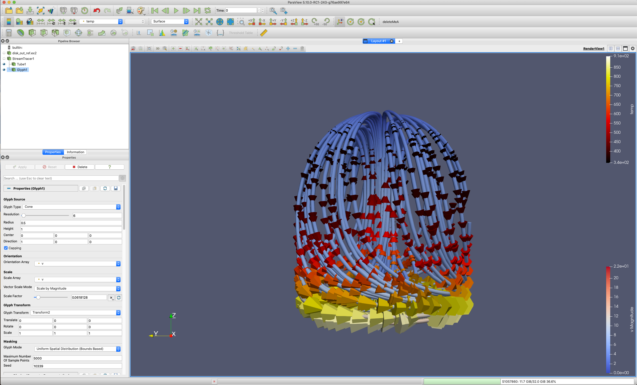
16.3. Stream Tracers - lines and tubes
Open disk_out_ref.ex2.
Apply.
+X
Select Filters → Common → Stream Tracer.
v.
Set Seed Type to Point Cloud.
Uncheck Show Sphere.
Set Coloring to v.
Apply.
Lines don’t color as nicely as surfaces. Lets add a tube filter around each streamline.
Select Filters → Search
Type Tube.
Apply.
Now, we want to know which directions the particles are moving. We will use a glyph filter. Note we place the glyph filter on the streamline, not the tube.
Select StreamTracer1 in the Pipeline Browser.
Select Filters → Common → Glyph.
Set Glyph Type to Cone.
Set Orientation Array to v.
Set Scale Array to v.
!Very Important!: In the Scale Factor select the recycle button to the right.
Apply.
Set Coloring to temp.
View → Color Map Editor → Presets (the little envelope with a heart) → Black Body Radiation.
Lets save this really cool image as a screenshot.
File → Save Screenshot.
Add a file name.
OK.
OK.
Edit → Reset Session.
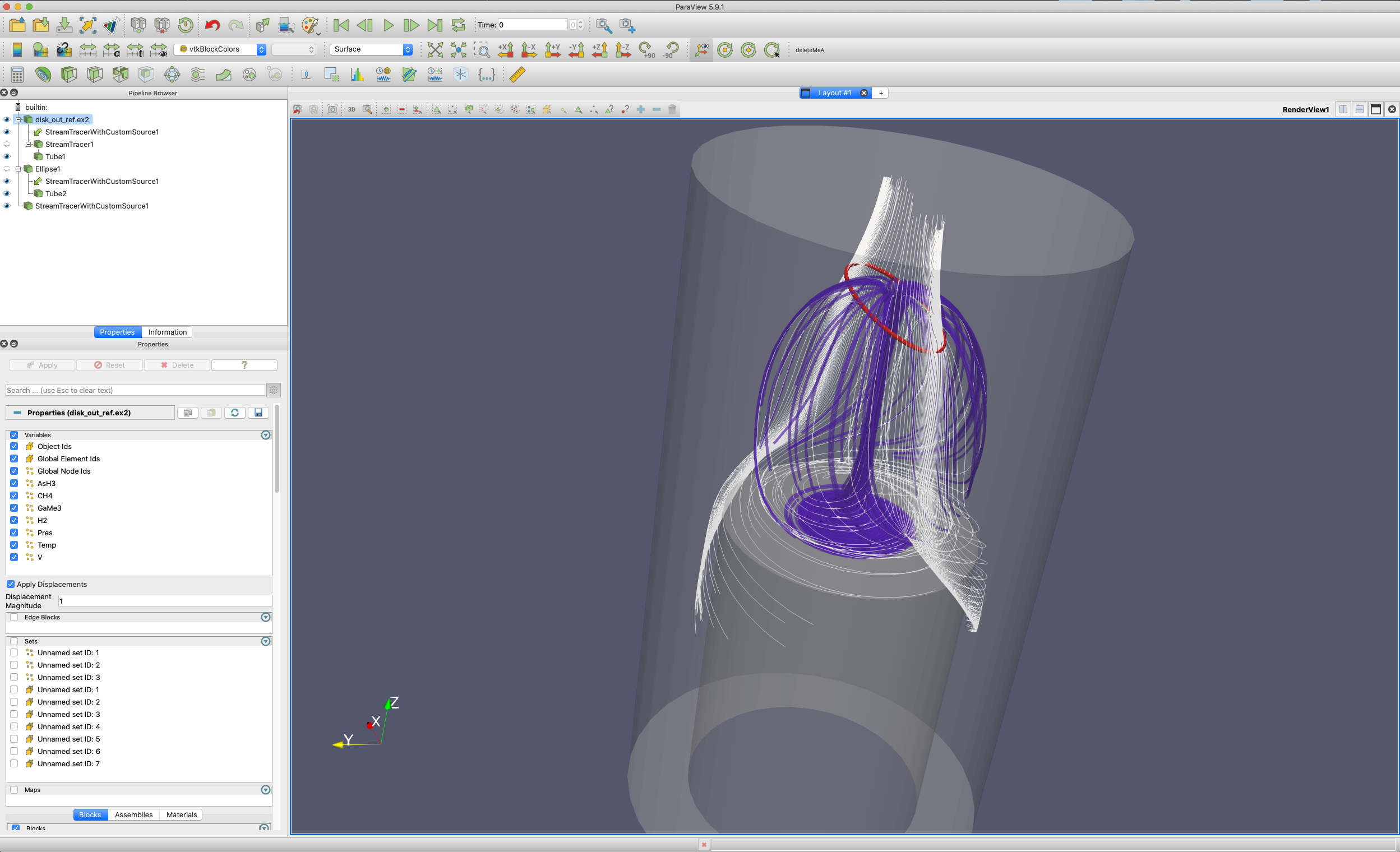
16.4. Stream Tracers with Custom Source
We want to create stream tracers from any arbitrary source. This can be a line, spline, circle, ellipse or any other curving line. An extreme example would be a cylinder cut by a plane.
Open disk_out_ref.ex2.
Apply.
+X
Set vtkBlockColors to Solid Color.
Set Opacity to 0.3.
Sources/Alphabetical/Ellipse.
Set Center to 0,0,7.
Set Major Radius Vector to 3,0,0.
Set Ratio to 0.3.
Apply.
Select Filters → Search
Type Tube.
Apply.
Select disk_out_ref.ex2 in the Pipeline Browser.
Select Filters → Alphabetical → Stream Tracer with Custom Source.
Set Seed Source to Ellipse.
Apply.
Set Coloring to Solid Color.
The image below is a merging of Stream Tracers with lines and tubes, and Stream Tracer with Custom Source. I have also played with colors to make it look nicer. If interested, replicating is left to the user.
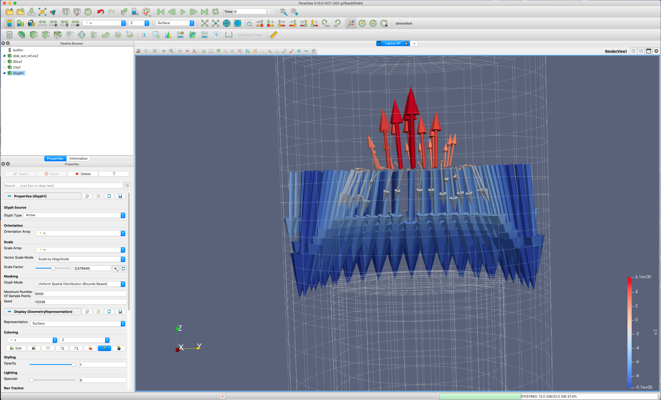
16.5. Glyphs perpendicular to a slice
Edit → Reset Session.
Open disk_out_ref.ex2.
Apply.
+X.
Lets create a half slice. This will be used as the seed plane for glyphs.
Select Filters → Common → Slice.
Z Normal.
Set Origin to 0, 0, 5.
Uncheck Show Plane.
Apply.
Select Filters → Common → Clip.
Uncheck Show Plane.
Apply.
Now, apply glyphs.
Select Filters → Common → Glyph.
Set Glyph Type to Arrow.
Set Orientation Array to v.
Set Scale Array to v.
!Very Important!: In Scale Factor select the recycle button to the right.
.5X.
.5X.
Apply.
Set Coloring to v.
Change Magnitude to Z.
Let’s put these glyphs back into context by showing the original dataset.
Select disk_out_ref.ex2 in the Pipeline Browser.
Set Representation to Wireframe.
In the pipeline browser, click on the eyeball next to disk_out_ref.ex2.
Set Opacity to 0.3.
Use the mouse to zoom into the glyph vectors.
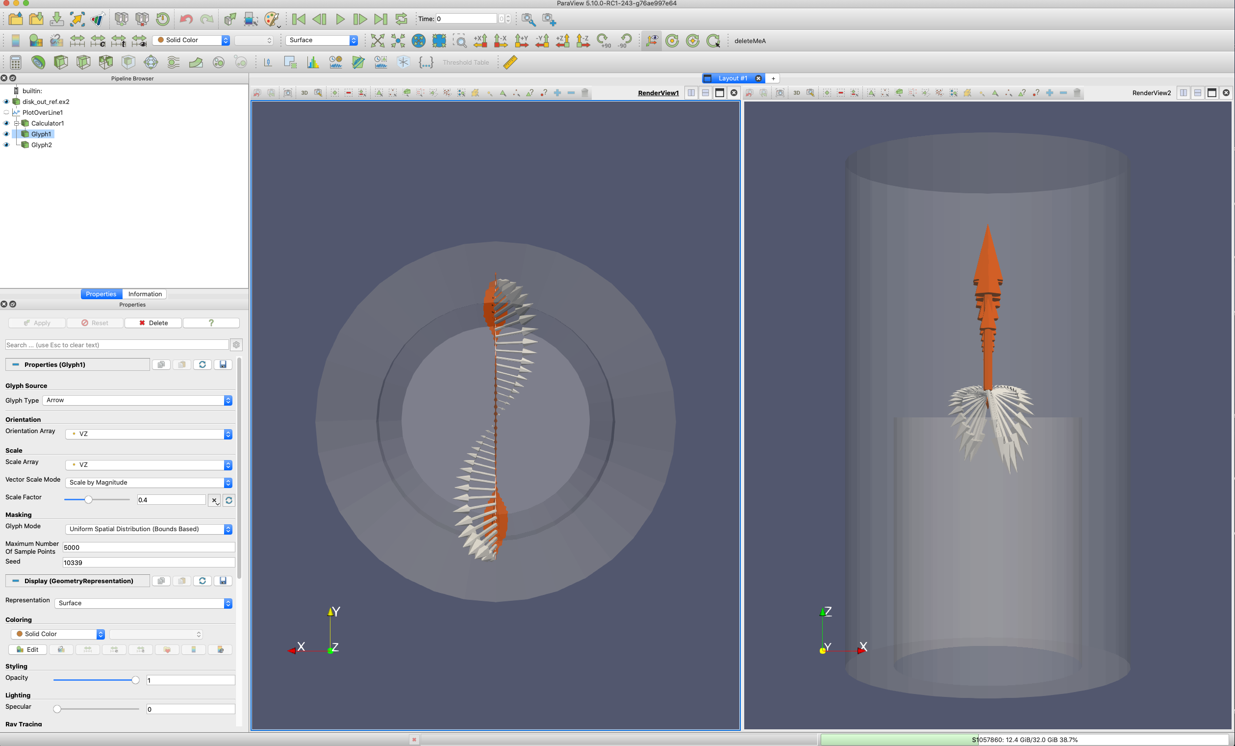
16.6. Flow in a fluid
To show a velocity profile we need to sample the dataset with a line, and then create glyphs off of this line. This can be done using a trick in ParaView, i.e., the Plot over Line filter. Note that a Resample to Line filter will be added in ParaView 5.11 or so.
Edit → Reset Session.
Open disk_out_ref.ex2.
Apply.
Lets sample over a line.
Select Filters → Domain → Data Analysis → Plot over Line.
Y Axis.
Change the Z component of Point1 and Point2 to 1.
Change the Resolution to 40.
Apply.
Close the LineChartView.
In the Pipeline Browser, turn visibility off for disk_out_ref.ex2.
We now have a line sampled through the fluid. Lets calculate the negative Z component of V (so it goes the opposite direction on the line from V). That way we can have two profiles, one with V, and one with Vz.
Make sure that PlotOverLine is selected
Set Filters → Common → Calculator.
Change Result to Vz.
Set Expression to 0*iHat+0*jHat+-v_Z*kHat.
Apply.
Now we want to create two Glyphs - one from the Calculator filter, and one directly from the Plot over Line filter.
Calculator1 should still be highlighted in the Pipeline Browser.
Select Filters → Common → Glyph.
Set Glyph Type to Arrow.
Set Orientation Array to Vz.
Set Scale Array to Vz.
!Very Important!: In Scale Factor select the recycle button to the right.
.5X.
.5X.
Apply.
Click on the Color Editor icon.
Change the color to Orange.
Apply.
In the Pipeline Browser select the Plot over Line filter.
Select Filters → Common → Glyph.
Set Glyph Type to Arrow.
Set Orientation Array to v.
Set Scale Array to v.
!Very Important!: In Scale Factor select the recycle button to the right.
Apply.
Let’s put these glyphs back into context by showing the original dataset.
Select disk_out_ref.ex2 in the Pipeline Browser.
Click on the eyeball next to disk_out_ref.ex2.
Set Opacity to 0.3.
Just to create a nice image, I’m going to split the views horizontally, and show this visualization also from the side.
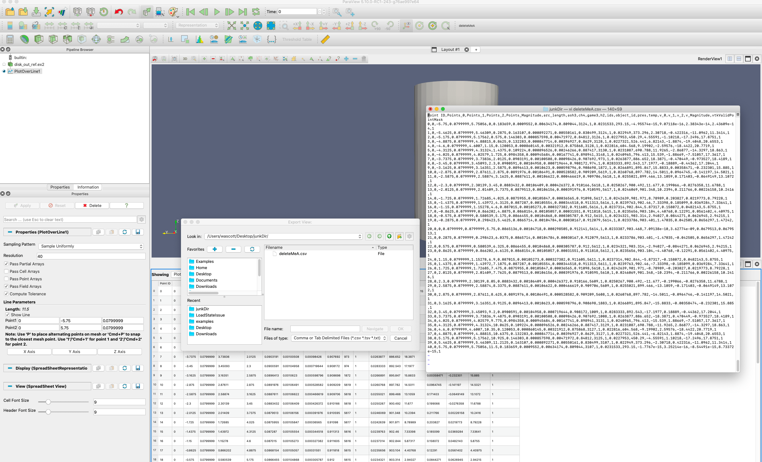
You can write the data sampled down the line to a .csv file, where you can post process it with tools such as Excel. Here is how to do it.
Select PlotOverLine in the Pipeline Browser.
Split screen vertical.
Spreadsheet view.
Now, click on the Export Spreadsheet icon, and write the Spreadsheet down to a .csv file.
Lets save this really cool image as a screenshot.
File → Save Screenshot.
Add a file name.
OK.
We want to save both views. Click Save All Views.
OK.
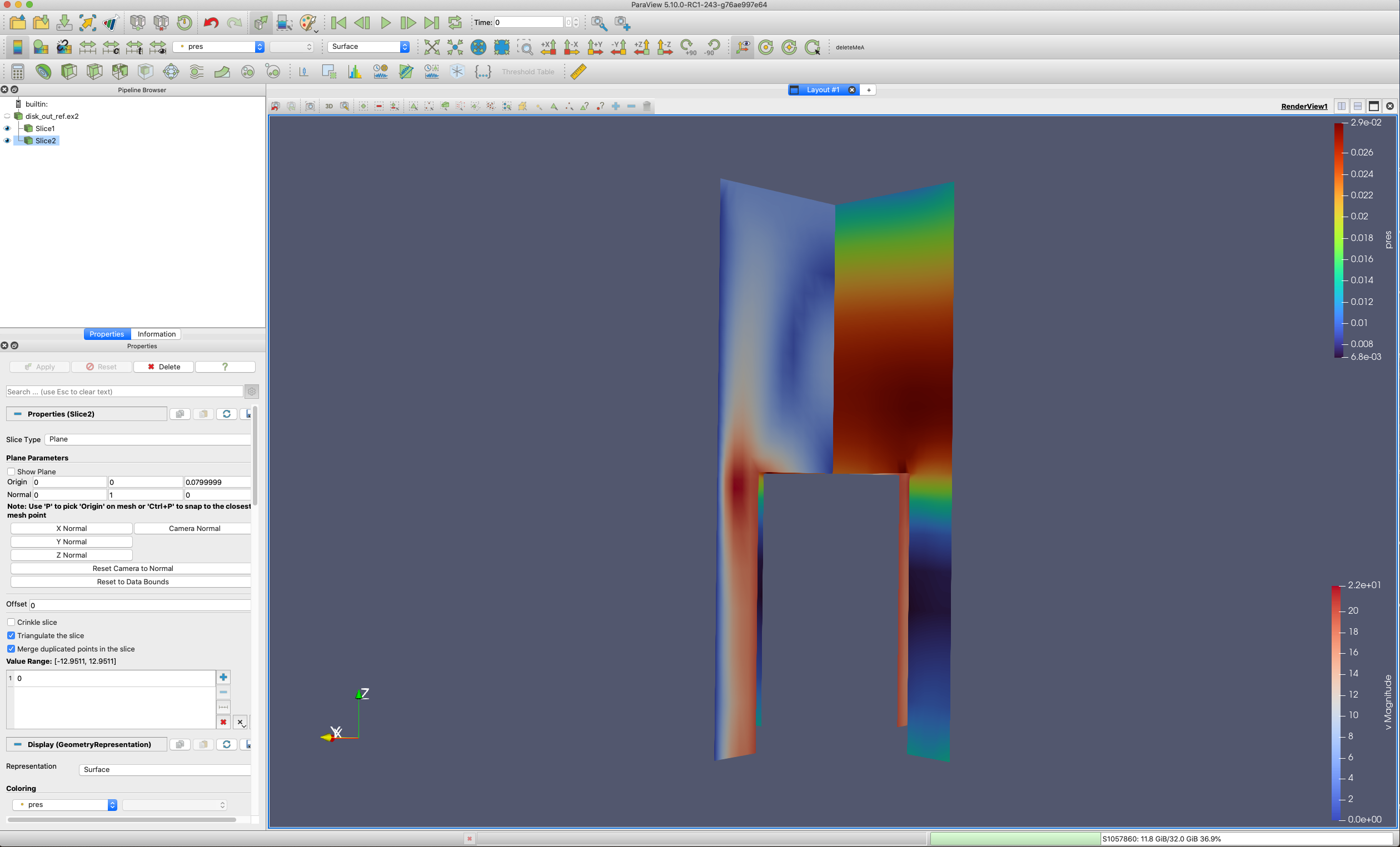
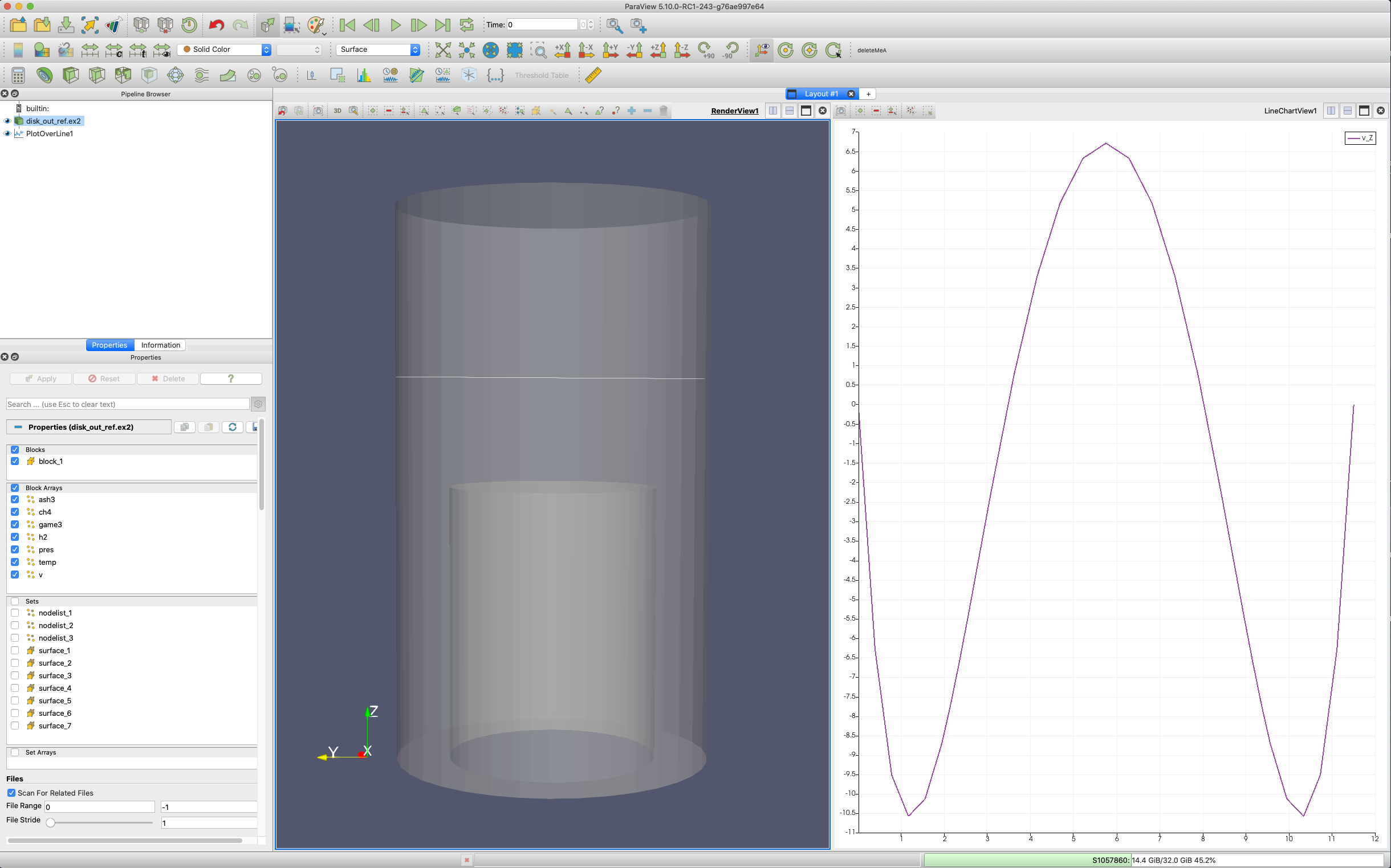
16.7. 2D plots through a fluid
Edit → Reset Session.
Open disk_out_ref.ex2.
Apply.
+X.
Select Filters → Domain → Data Analysis → Plot over Line.
Y Axis.
Change the Z component of Point1 and Point2 to 4.
Apply.
In the Properties Tab, turn all variables off other than v_Z.
Click on the RenderView, the left view.
Select disk_out_ref.ex2 in the Pipeline Browser.
Set Opacity to 0.3.
16.8. Contours on a slice
Edit → Reset Session.
Open disk_out_ref.ex2.
Apply.
+X.
Select Filters → Common → Slice**.
Uncheck Show Plane.
Apply.
We need the magnitude for the Contour filter.
Select Filters → Common → Calculator**.
Result Array Name vMag.
Set Expression to mag(v).
Apply.
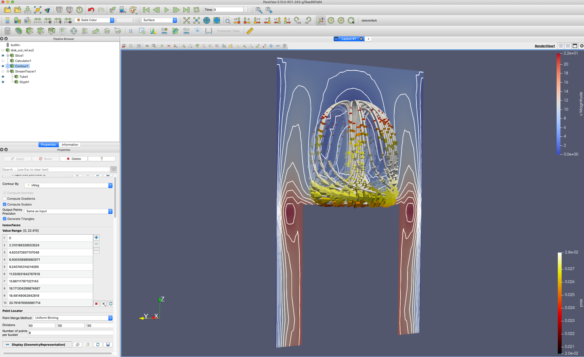
Now, draw contours on the 2d slice.
Select Filters → Common → Contour.
Contour by vMag.
Delete the Value, and create a new set using the Add a Range of Values icon.
Apply.
A nice visualization is to turn visibility on for Slice and paint by v, and change Contour to be a Solid Color, and make that color White.
Here is an example with additional streamlines, tubes and glyphs.
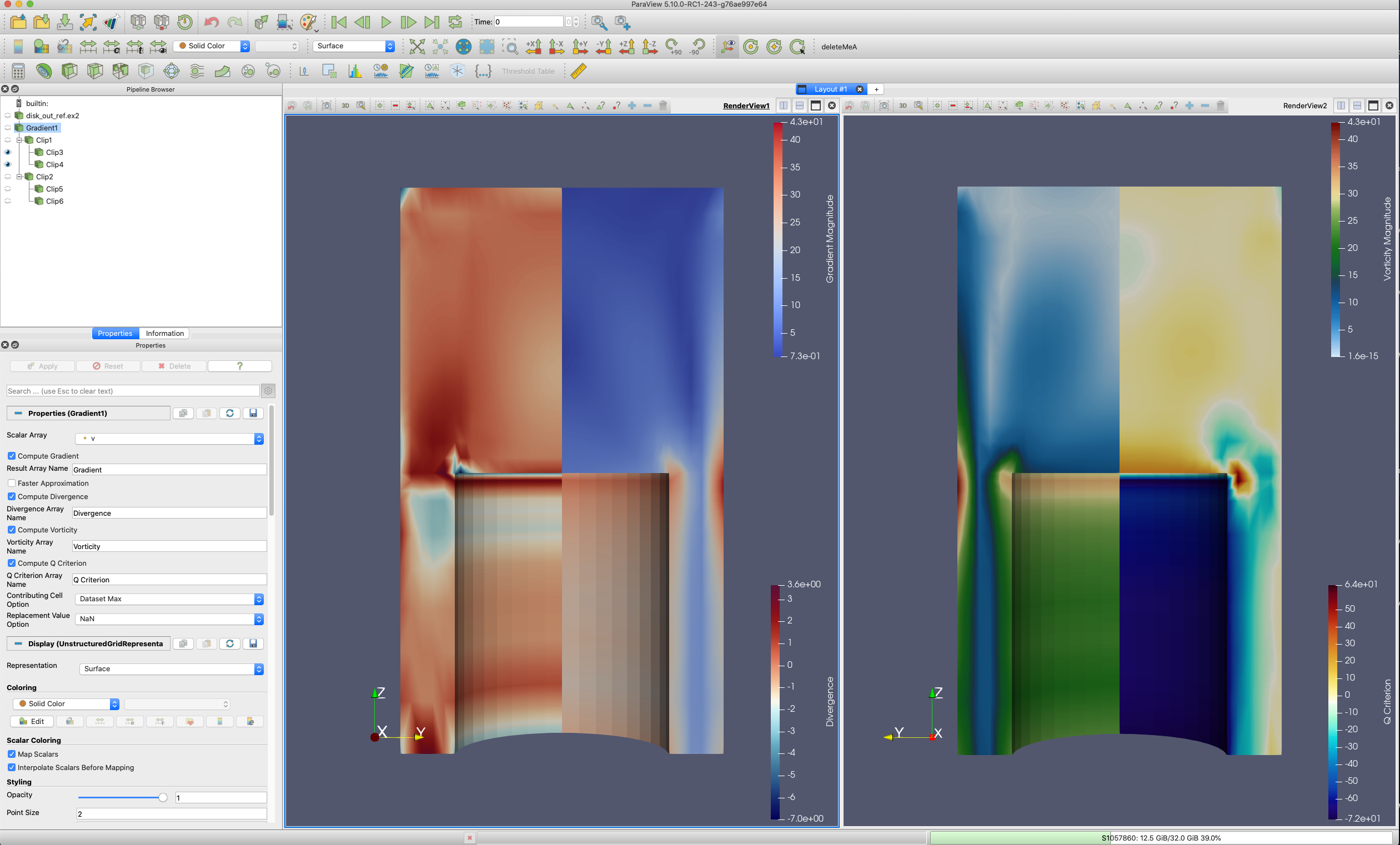
16.9. Gradient, Divergence, Vorticity and Q Criterion
The Gradient filter (Advanced Properties tab) provides Gradient, Divergence, Vorticity and and Q Criterion. Here is am example, using disk_out_ref.ex2.
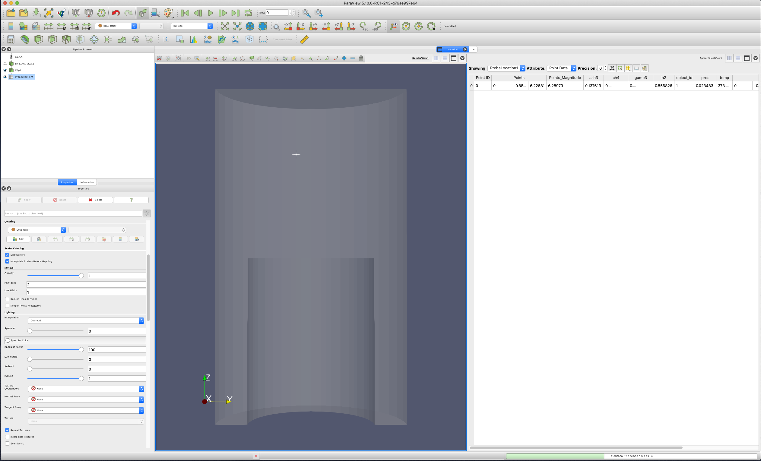
16.10. Probing a fluid
There are numerous ways to probe the cells and points of a fluid. One is with the Hover Points On and Hover Cells On icons just above the Renderview. Another is with Interactive Select Cells or Points On. Then, in the Find Data, turn on Cell or Point Labels. Yet another is with the Probe filter. Here is how to use the probe filter.
Edit → Reset Session.
Open disk_out_ref.ex2.
Apply.
+X.
Select Filters → Common → Clip.
Uncheck Show Plane.
Uncheck Invert.
Apply.
The Probe filter works much better with Auto Apply turned on. This is the icon that looks like a tree growing out of a cube.
Auto Apply on
Select Filters → Domain → Data Analysis → Probe.
If needed, select the RenderView window, giving it focus.
Now, move over disk_out_ref.ex2, updating the probed location with the p key. The probed data will show in the Spreadsheet view.
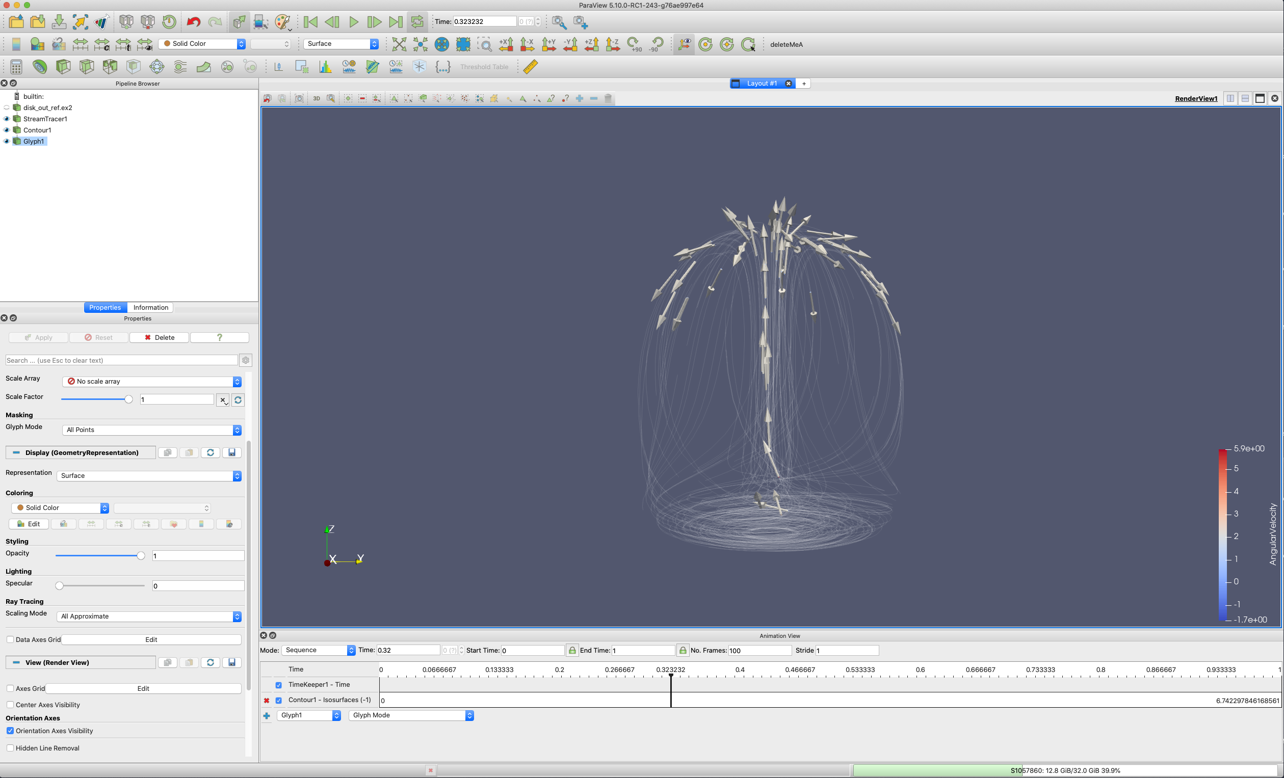
16.11. Animating a static vector field
If you have a vector field in your data, you can animate a static dataset. Our goal is to create a set of streamlines from a vector field, place points on this set of streamlines, and animate the point down the streamlines. We will also add glyphs to the streamline points.
Edit → Reset Session.
Open disk_out_ref.ex2.
Apply.
Click the -X icon.
Stream tracer filter. (We are already streamtracing on V).
Set Seed Type to Point Cloud.
Optional - change the Opacity to 0.4.
Apply.
Select Filters → Common → Contour.
Contour on IntegrationTime.
Apply.
Select Filters → Common → Glyph.
Vectors V.
No Scale Array.
Scale 1.
Set Glyph Mode to All Points.
Apply.
Select View → Animation View.
Set Mode to Sequence.
Set No. Frames to 100.
Change the pulldown box next to the blue + to be Contour.
Click the blue +. Note it works better if you use 0 for the start.
Now, click the play button.
In the pipeline browser, I also turned off visibility for the Contour filter.
Lets save this as a movie.
File → Save Animation.
Add a file name.
Save as a .avi.
OK.
OK.
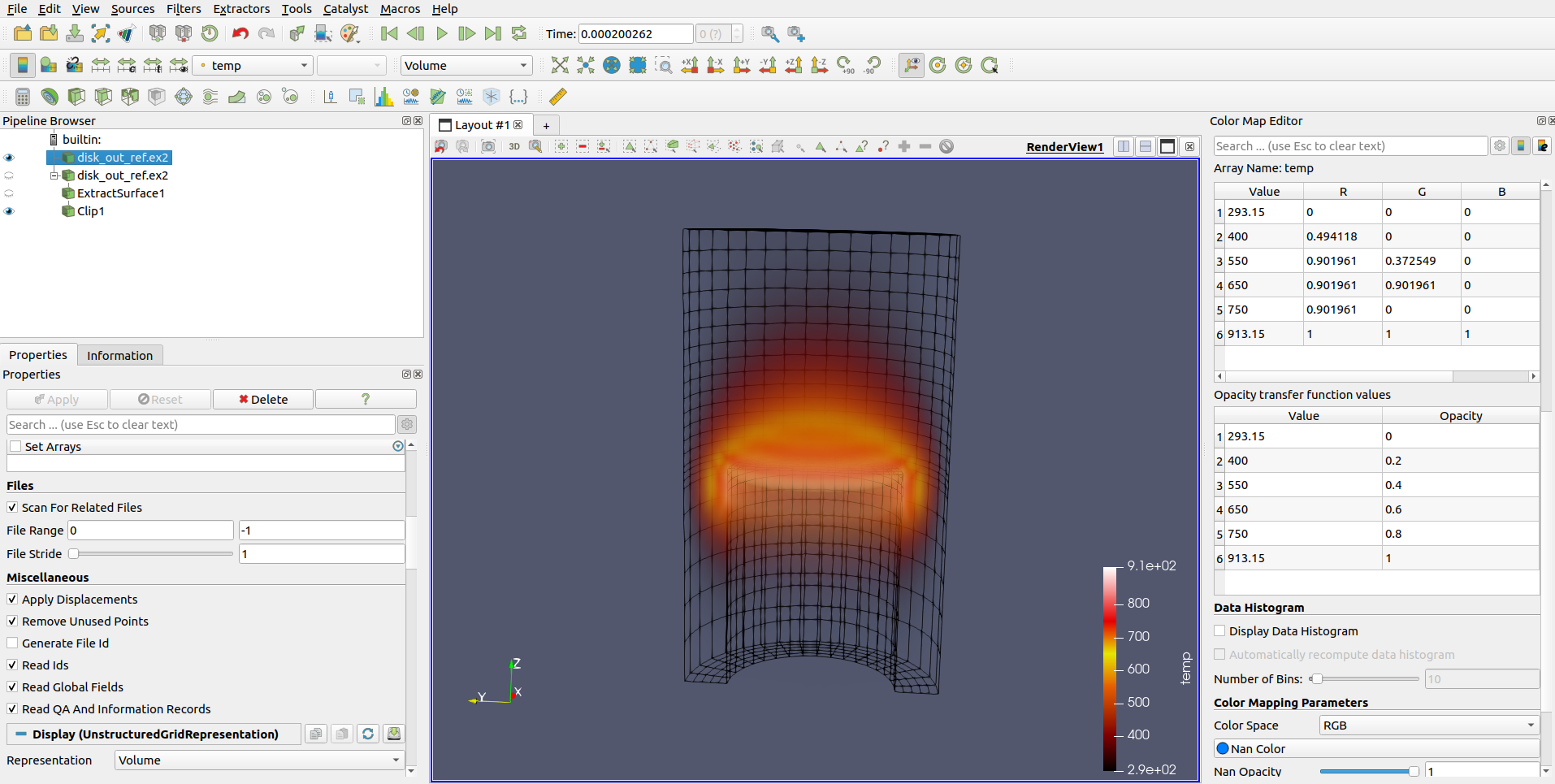
16.12. Volume Rendering
We are going to paint the fluid by volume rendered temperature and we will try to make it look like fire. To give context, we are also going to extract the exterior surface, and clip the disk_out_ref in half. We will paint this exterior surface black.
Note: Volume rendering is very resource intensive. It is possible to display a dataset using surface that chokes using Volume Rendering. The solution is to grab more nodes of your cluster, thus picking up more memory.
Edit → Reset Session.
Open disk_out_ref.ex2
Apply.
Select Filters → Alphabetical → Extract Surface.
Apply.
Select Filters → Common → Clip.
Deselect Invert.
Apply.
Set Solid Color to black.
Set Representation to Wireframe.
Open disk_out_ref.ex2 again.
Apply.
Set Coloring to temp.
Set Representation to Volume.
Since the goal is to make it look like fire, we will finetune the Color Map settings.
Select View → Color Map Editor
Change presets (looks like a folder with a heart) to be Black Body Radiation.
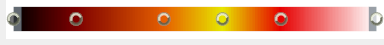
The Color Transfer function (the lower 1D colored line) should already have 4 points.
Add a point in the orange area
Add another at the top of the black.
Did you know?
You can create a point on the color scale by clicking in the window.
You can select a point on the color scale by clicking on it.
You can move between points using the Tab and Shift keys.
You can delete points using the delete key.
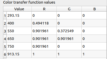
The temperature should be set by the physical laws of black body curve. Thus, manually specify the color transfer function values of the 6 points as follows by clicking the advanced button.
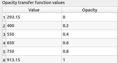
The Opacity Transfer function (the upper 2D colored line) should already have 2 points.
Add 4 extra points as seen below.
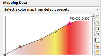
The Opacity requires a bit of artistic license. What we are trying to do is show the different temperatures inside of the flame. Also, we may want to show differing amounts of soot - which will be point number1. Thus, manually specify the opacity transfer function values of the 6 points as follows.
The end result of the volume rendered fire should look like this: