17. Targeted: Particle Simulations
17.1. Introduction
Particle simulations consist of point data, rather than cell or element data. An example may be electrons in a field, or water molecules in a fluid. Particle datasets can be combined with other datasets to show particle motion in a solid or liquid.
This tutorial uses a dataset named mediumVector.vtu. I will try to get it on the Kitware web site. If you want to make it yourself, it is just a vtk dataset, using the format listed at the end of this tutorial. I then read it into ParaView, and used the reflect filter in the X, then Y, then Z direction. I believe I then did the same reflections again. Finally, this file was written out to disk as a .vtu file.
17.2. Displaying particles
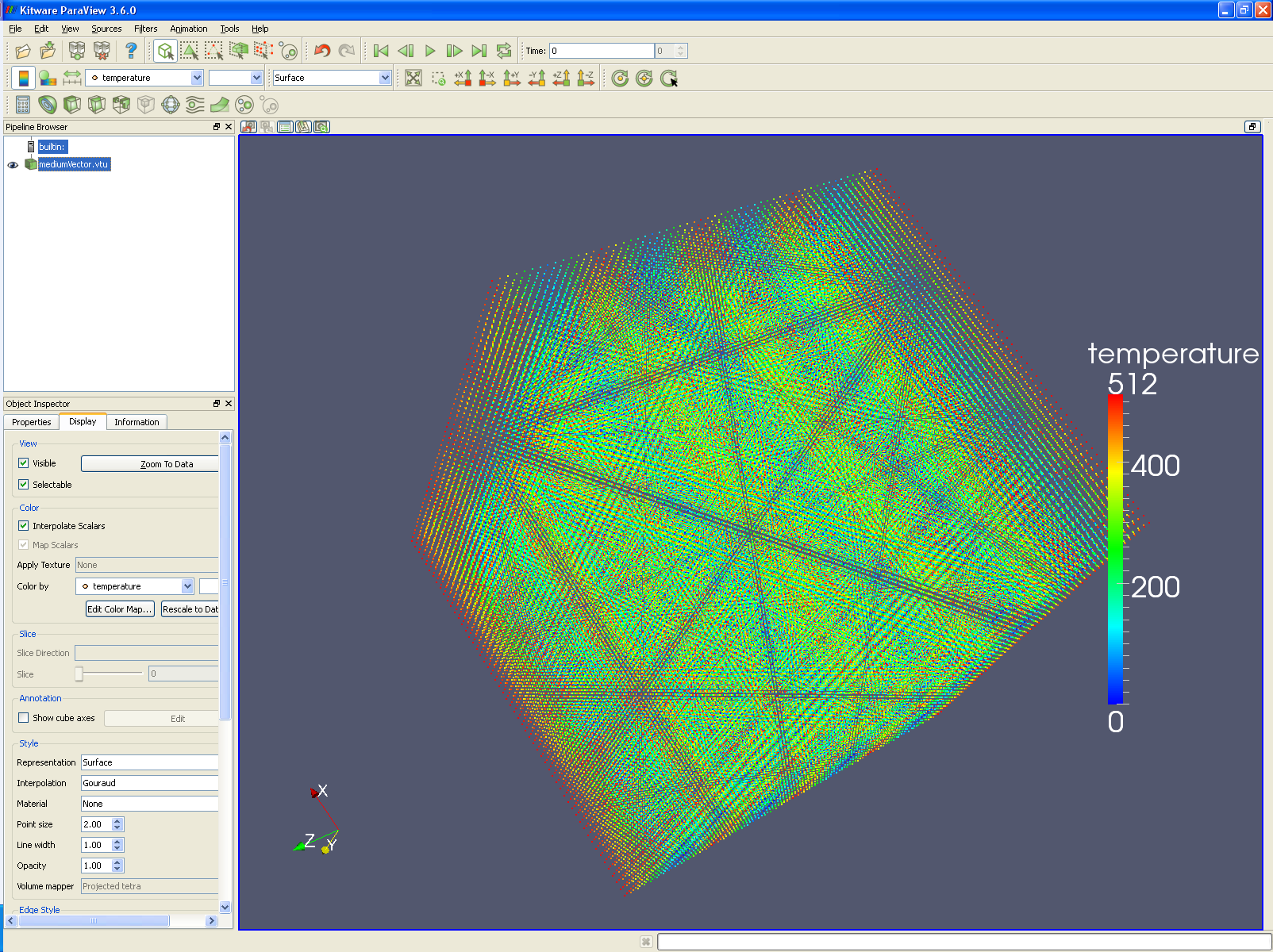
Run
paraview.Open mediumVector.vtu.
In the Properties tab, set the Point size to 2 (or 1, depending on your preference). The following picture holds about 250,000 points.
17.3. Glyphing particles
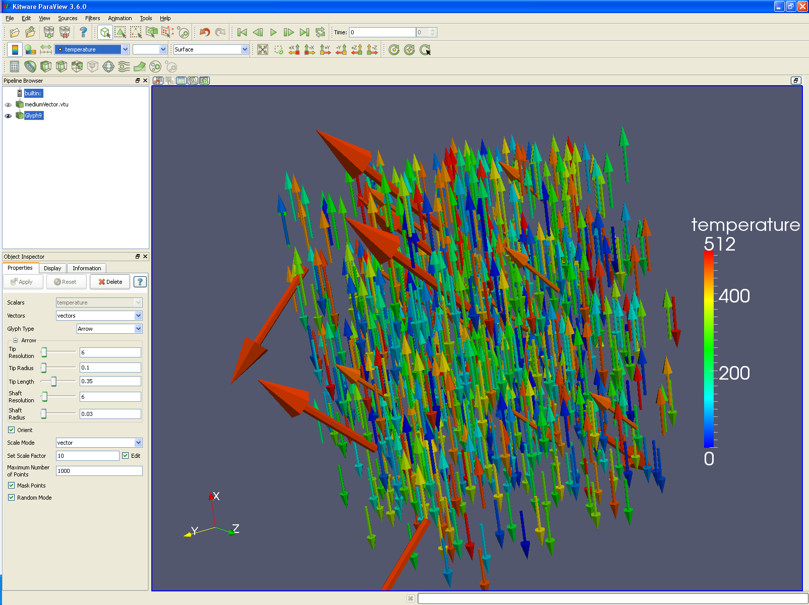
You may want to replace these particles with spheres or arrows, using the glyph filter. The glyph filter will depopulate your dataset to a reasonable number of items, and this reasonable number is set by the Maximum number of points input box. Random mode often creates better looking output, but is not useful if you animate through numerous time steps. The following picture has arrows for particles, using vectors for direction and length, and colored by temperature.
17.4. Thresholding particles
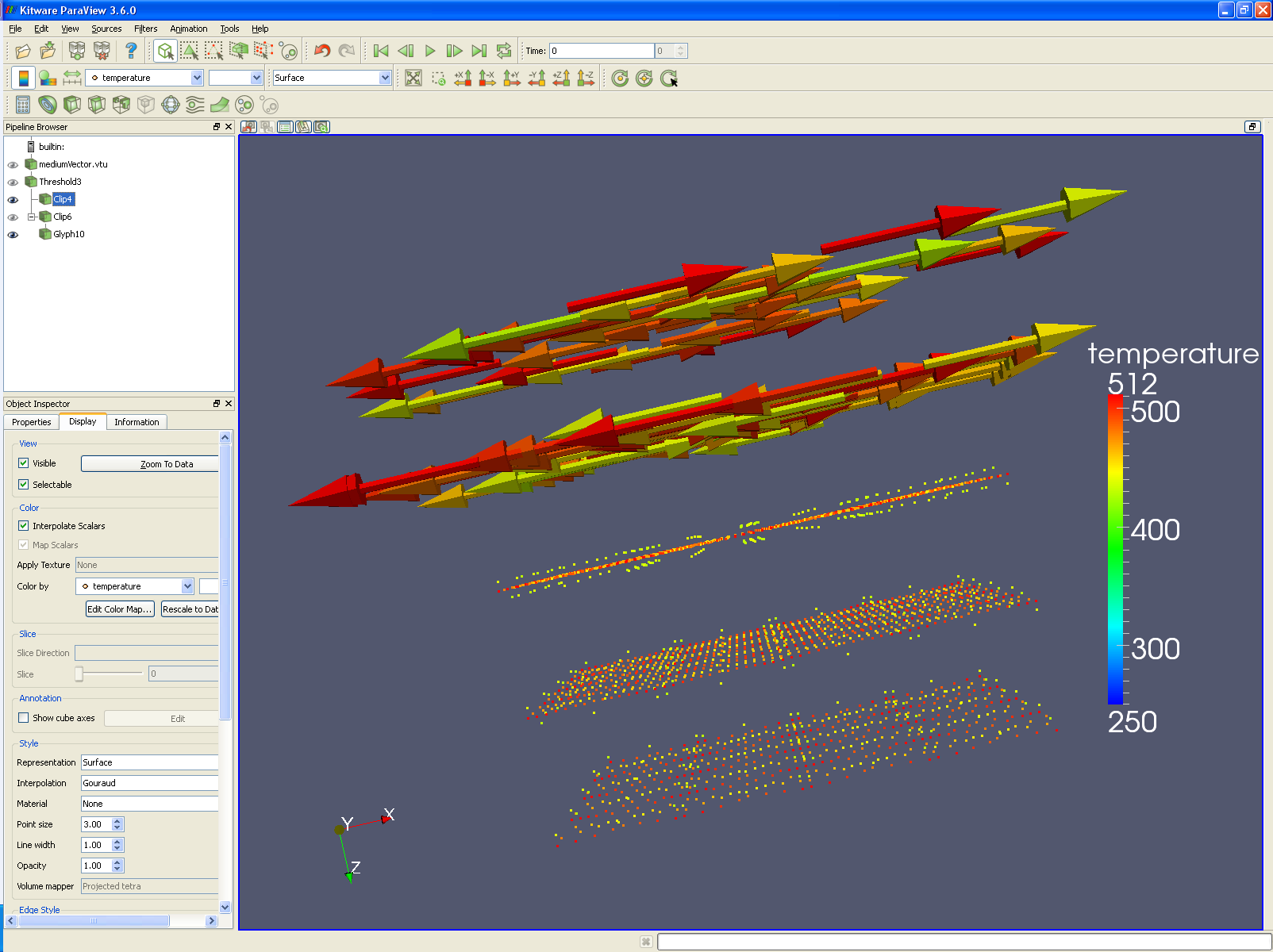
Another filter that is useful is the Filters → Alphabetical → Threshold. Using the Threshold filter, a user can select only those particles that are of interest. For instance, the following picture only displays particles that have a temperature of 430 to 511 degrees. Using the Filters → Common → Clip, the upper half of the picture has arrow glyphs, and the lower half has the particles themselves - all colored by temperature.
17.5. Scatter Plot
Finally, you can make a scatter plot through the Filters → Common → Calculator. For instance, if we want to preserve the X and Y coordinates of our points, but use number of pizzas for the Z component, we would do the following:
Select Filters → Common → Calculator.
Check the Coordinate Results check box.
Set Expression to coordsX*iHat+coordsY*jHat+pizza*kHat. This creates a vector, as follows: (X,Y,pizzas). (Think of the iHat as “This is an X”, the * as tying the coordinates and variables together, and the + sign as the comma between X,Y, and Z.)

17.6. Example data file
This data is written to a .vtk file. Note that I have deleted a lot of the data, which will need to be recreated. Also note that I added some random variable data - for instance, some locations have 1 or 2 pizzas. This actually creates a strange dataset - with many points per cell, but it worked for display purposes.
# vtk DataFile Version 2.0
Unstructured Grid Example
ASCII

DATASET UNSTRUCTURED_GRID
POINTS 512 float
0 0 0  1 0 0  2 0 0  3 0 0  4 0 0  5 0 0  6 0 0  7 0 0
0 1 0  1 1 0  2 1 0  3 1 0  4 1 0  5 1 0  6 1 0  7 1 0
...
0 0 1  1 0 1  2 0 1  3 0 1  4 0 1  5 0 1  6 0 1  7 0 1
0 1 1  1 1 1  2 1 1  3 1 1  4 1 1  5 1 1  6 1 1  7 1 1
...
0 0 2  1 0 2  2 0 2  3 0 2  4 0 2  5 0 2  6 0 2  7 0 2
0 1 2  1 1 2  2 1 2  3 1 2  4 1 2  5 1 2  6 1 2  7 1 2
...
CELL_TYPES 52
1
1
...
POINT_DATA 512
SCALARS temperature float 1
LOOKUP_TABLE default
000.0 001.0 002.0 003.0 004.0 005.0 006.0 007.0 008.0 009.0
010.0 011.0 012.0 013.0 014.0 015.0 016.0 017.0 018.0 019.0
...
SCALARS pizza float 1
LOOKUP_TABLE default
000.0 000.0 000.0 000.0 000.0 000.0 000.0 000.0 000.0 000.0
000.0 000.0 000.0 000.0 000.0 000.0 000.0 000.0 000.0 000.0
...
VECTORS vectors float
1 0 0  1 0 0  1 0 0  1 0 0  1 0 0  1 0 0  1 0 0  1 0 0  1 0 0  1 0 0
1 0 0  1 0 0  1 0 0  1 0 0  1 0 0  1 0 0  1 0 0  1 0 0  1 0 0  1 0 0
...