15. Targeted: ParaView & CTH
15.1. Introduction
This tutorial shows how to visualize CTH datasets (called spcth files). CTH is a multi-material, large deformation, strong shock wave, solid mechanics code developed at Sandia National Laboratories. A more complete writeup on CTH is here: http://www.sandia.gov/CTH/. CTH Spyplot files are Eulerian, or structured mesh datasets. They can be flat mesh or adaptive mesh refinement (i.e., AMR).
15.2. ParaView’s CTH reader
paraview reads spcth files in an very efficient manor. All material
volume arrays go from 0 (representing 0%) to 1 (representing 100%).
These are actually stored in the files as floats (4 bytes) or doubles (8
bytes). paraview reads these into unsigned bytes, which range from 0 to
255. Generally, you want a surface (contour or clip by scalar) at about
10%.
15.3. Creating contours with the Extract CTH Parts filter
Our goal is to create a contour where Material Volume Fractions is at 10%.
Start
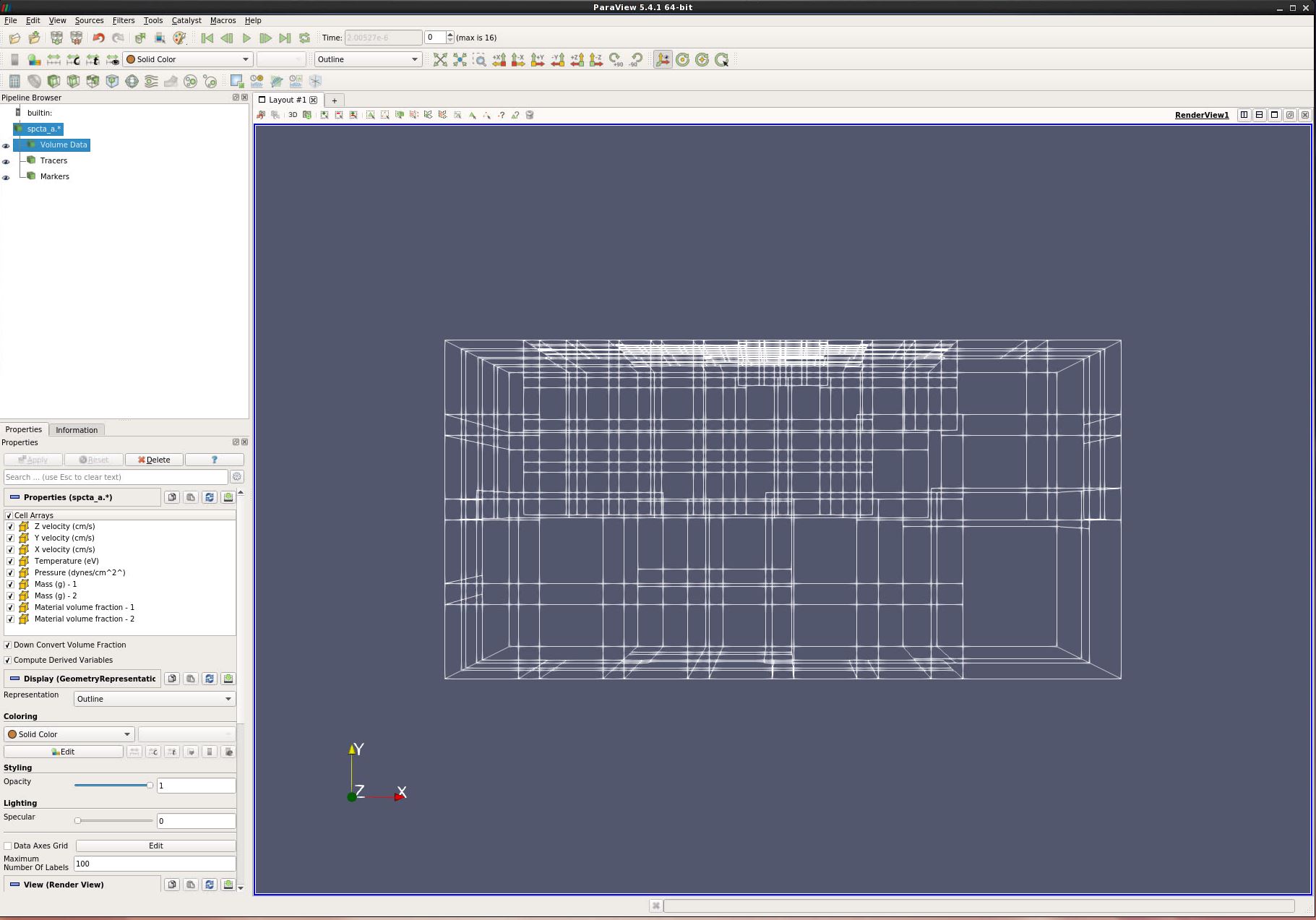
paraview.Open spcth_a.0.[0-3].
Turn all variables on.
Apply.
Notes:
There are three types of data that have been read in.
Volume data is the structured data from the CTH simuliation
Tracers are points in the mesh that move with a material, and can include variable information.
Markers are groups of points that move with a material.
Notice the Down Convert Volume Fraction has been checked. This means that ParaView will store volume fractions as an unsigned byte.
Y-
Note: Since we will have two materials touching each other, our default Volume Fraction Value will have some cells visible on top of each other. If this is not desired, change the value to 0.5.
Coloring by point will be smoother than color by cell. Thus, we will convert variables to be point for anything we color.
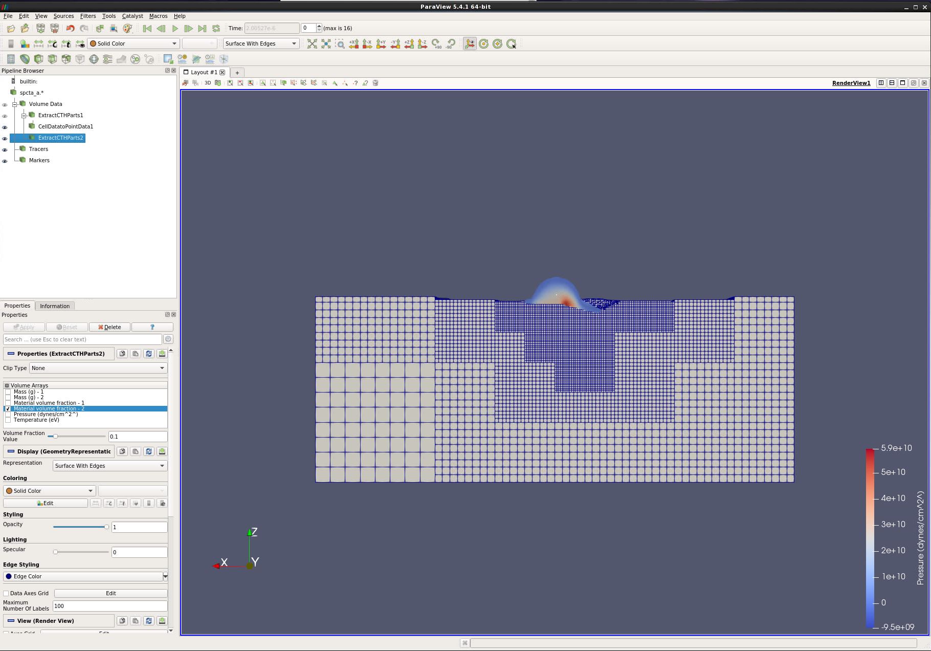
Filters/CTH/Extract CTH Parts.
Turn off all Volume Arrays, except Material volume fraction - 1.
Apply.
Filters → Alphabetical → Cell Data to Point Data.
Apply.
Set Coloring to Pressure.
In the Pipeline Browser, select Volume Data (i.e., the raw cth data again).
Filters → CTH → Extract CTH Parts.
Turn off all Volume Arrays, except Material volume fraction - 2.
Apply.
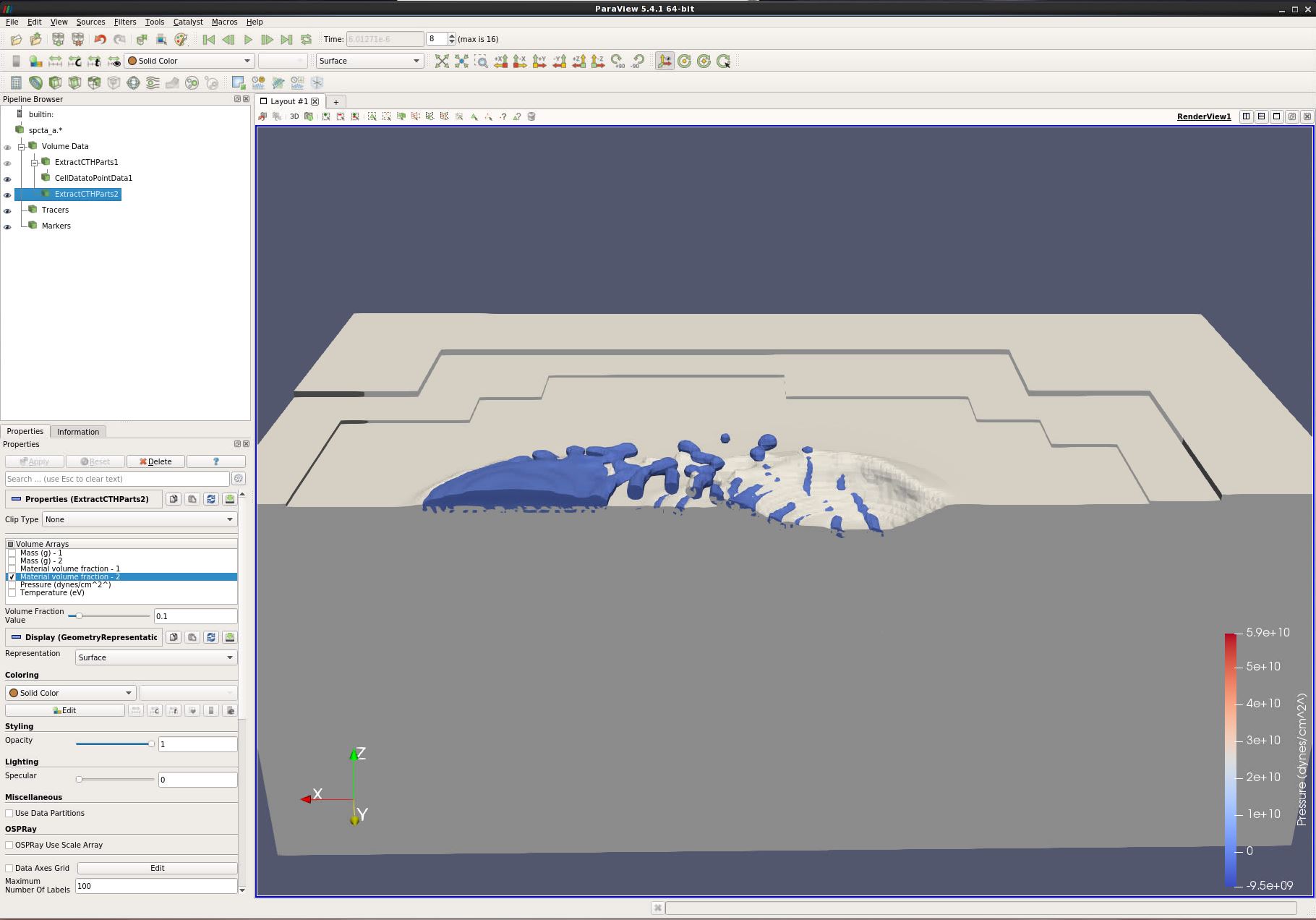
Change Representation to “Surface With Edges”.
Change Representation back to “Surface”.
With the left mousebutton, grab the 3d view and drag down. This will rotate the block face down.
With the right mousebutton, grab the 3d view and drag down. This will move closer to the block face.
Play forward to about the 8th timestep.
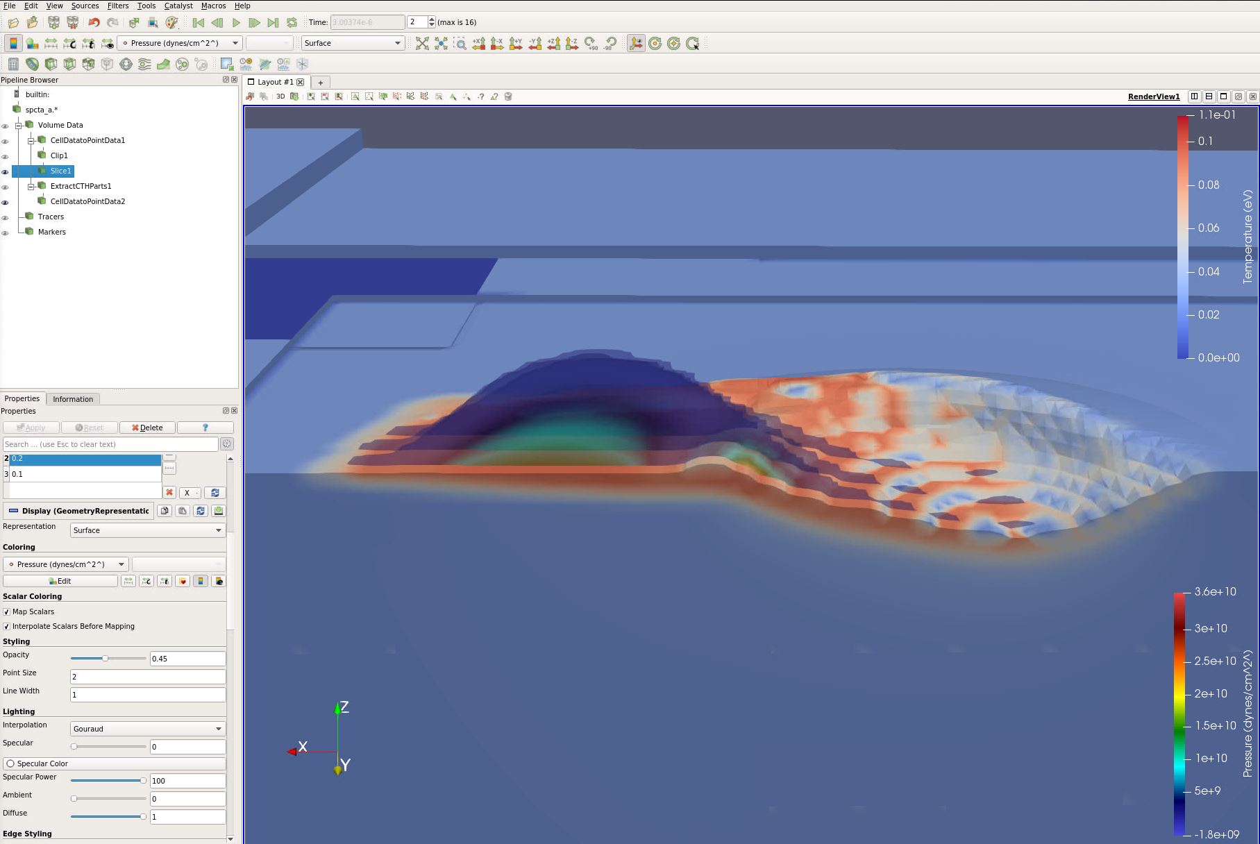
15.4. Creating a filled isovolume with the Clip by Scalar filter
Our goal is to create a solid 3d isovolume where Material Volume Fractions is at 10%. We want to do this so we can then take slices through the object.
Lets start from scratch.
Edit → Reset Session.
Open spcth_a.0.[0-3].
Turn all variables on.
Apply.
We now want to move our data to point based, as opposed to cell based data.
Filters → Alphabetical → Cell Data to Point Data.
Apply
We now extract one material volume. ParaView has actually read in Material volume fraction data as an unsigned byte, running from 0 to 255. 10% full is about 25, 50% is 128. Lets create an isovolume at 10%.
Filters → Common → Clip.
Set Clip Type to Scalar.
Set Scalars to Material volume fraction - 1.
Set Value to 25.
Apply.
Turn off visibility of the Cell Data to Point Data filter.
Filters → Common → Slice.
Y Normal.
Apply.
Unselect the Show Plane check box.
Set Coloring to Pressure.
We now want to change the colormap.
View → Color Map Editor. (There is a shortcut icon below the Edit menu.)
Click the Preset icon (little folder with a heart).
Rainbow Desaturated.
Apply.
Close.
Click Rescale to Custom Data Range (small icon below Sources).
Set range from 0 to 2e10.
Select the Volume Data in the pipeline browser.
Filters → CTH → Extract CTH Parts.
Select only Material volume fraction - 2.
Apply.
Filters → Alphabetical → Cell Data to Point Data. (This will smooth out the colors on each cell.)
Apply.
Set Coloring to Temperature (eV)
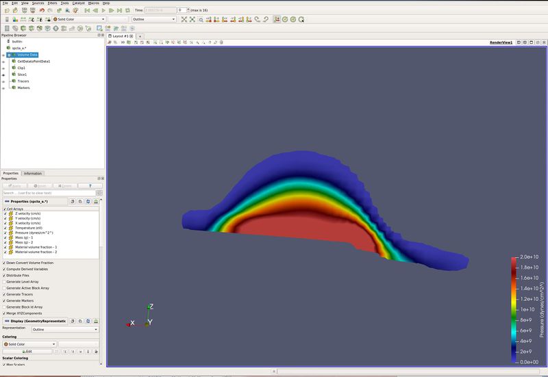
This image has three slices, opacity turned to 0.5 and the Extract CTH Parts filter is being painted by temperature.
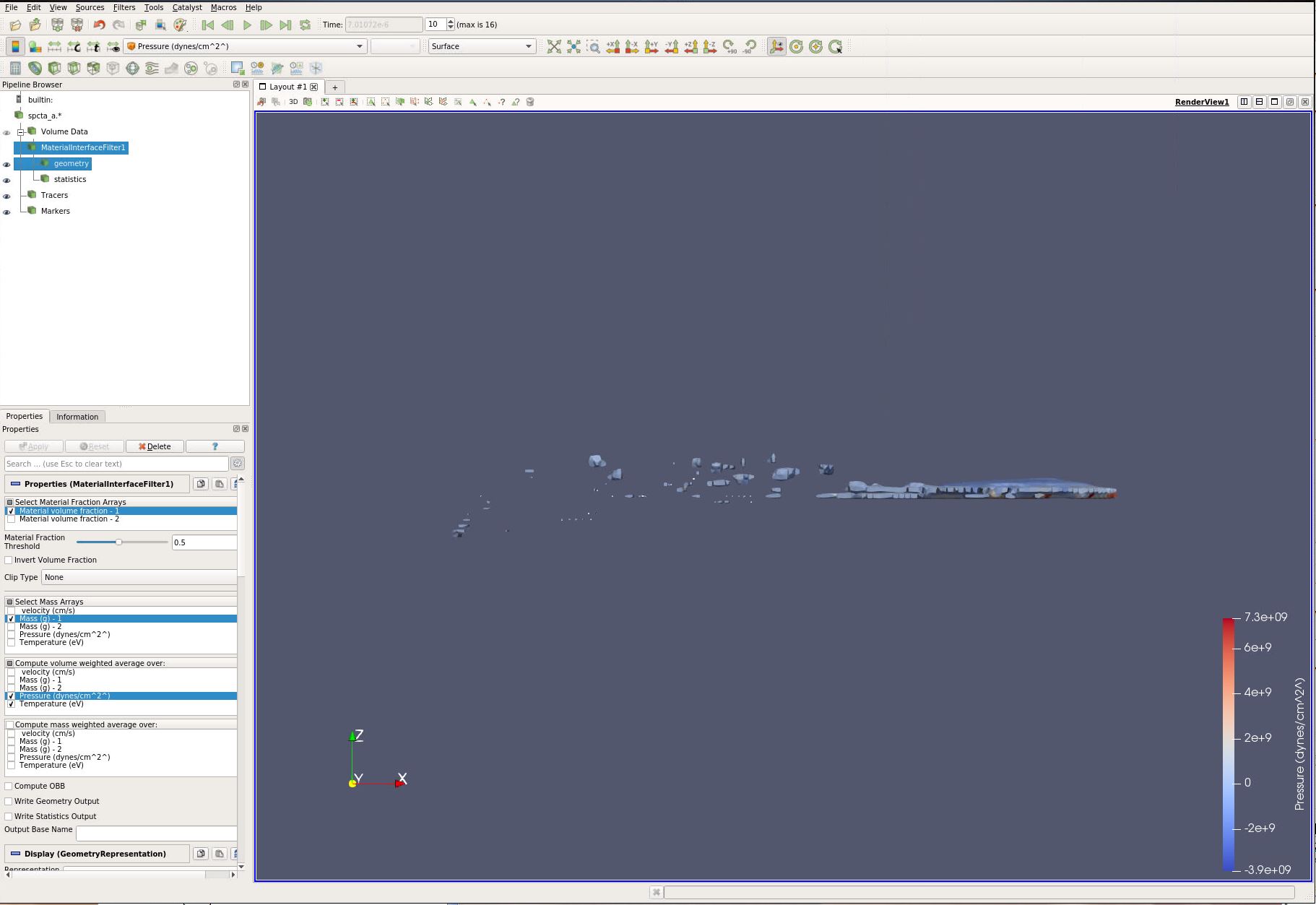
15.5. Analyzing fragments with the Material Interface filter
Our next goal is to analyze the fragments created by this simulation. To do this, we use the Material Interface Filter.
Lets start again from scratch.
Edit → Reset Session.
Open spcth_a.0.[0-3].
Turn all variables on.
Apply.
This filter is tricky. Do exactly as follows.
Filters → CTH → Material Interface Filter.
In Select Material Fraction Arrays select Material volume fraction - 1 (which is the ball).
In Select Mass Arrays select Mass (g) - 1 (which is the mass array for Material volume fraction - 1).
In Compute volume weighted average over select Pressure and Temperature.
Leave Compute mass weighted average over empty.
Apply
Go to the 10th timestep.
Paint by Pressure.
+Y
Turn off visibility for the geometry in the Pipeline Browser. This is done by clicking the eyeball.
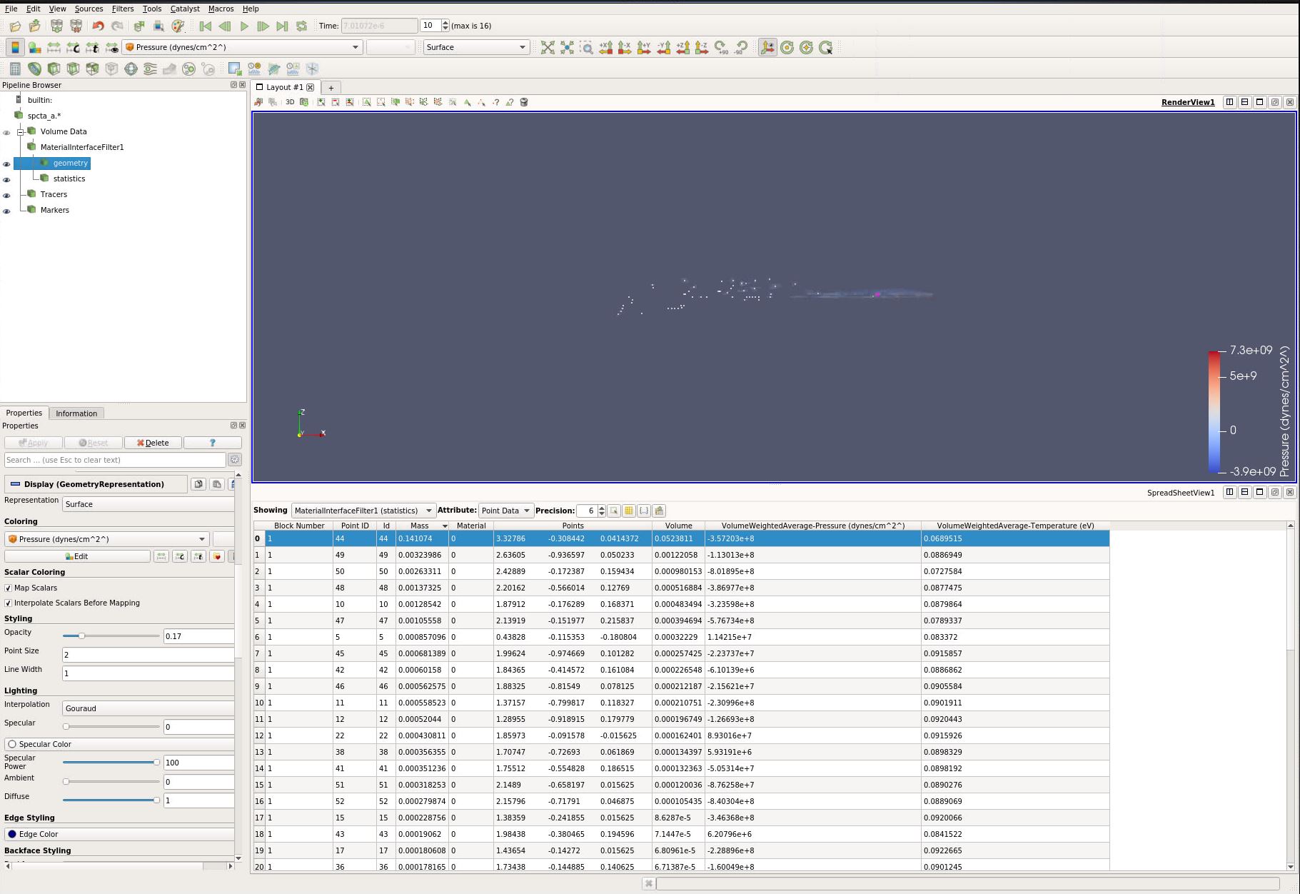
Anywhere there is a dot is the center of a fragment. We have statistics for each of these fragments.
Turn on visibility for the geometry in the Pipeline Browser.
Now, lets look at the statistics in the spreadsheet view.
split vertical. (This icon is found in the upper right corner of the 3d window)
Spreadsheet View
In the Pipeline Browser, click the eyeball for statistics
Each row represents a fragment.
In the Spreadsheet View, click on the Mass column. You have now sorted the spreadsheet.
The biggest fragment is the top row.
Click on the top row. It is now selected in the 3d view above.
Click in the 3d view, then turn off visibility for the geometry in the Pipeline Browser. The geometry of the fragment is hiding the selected statistic point.
Note that you can also change the opacity of the geometry, so you can see this selected point.
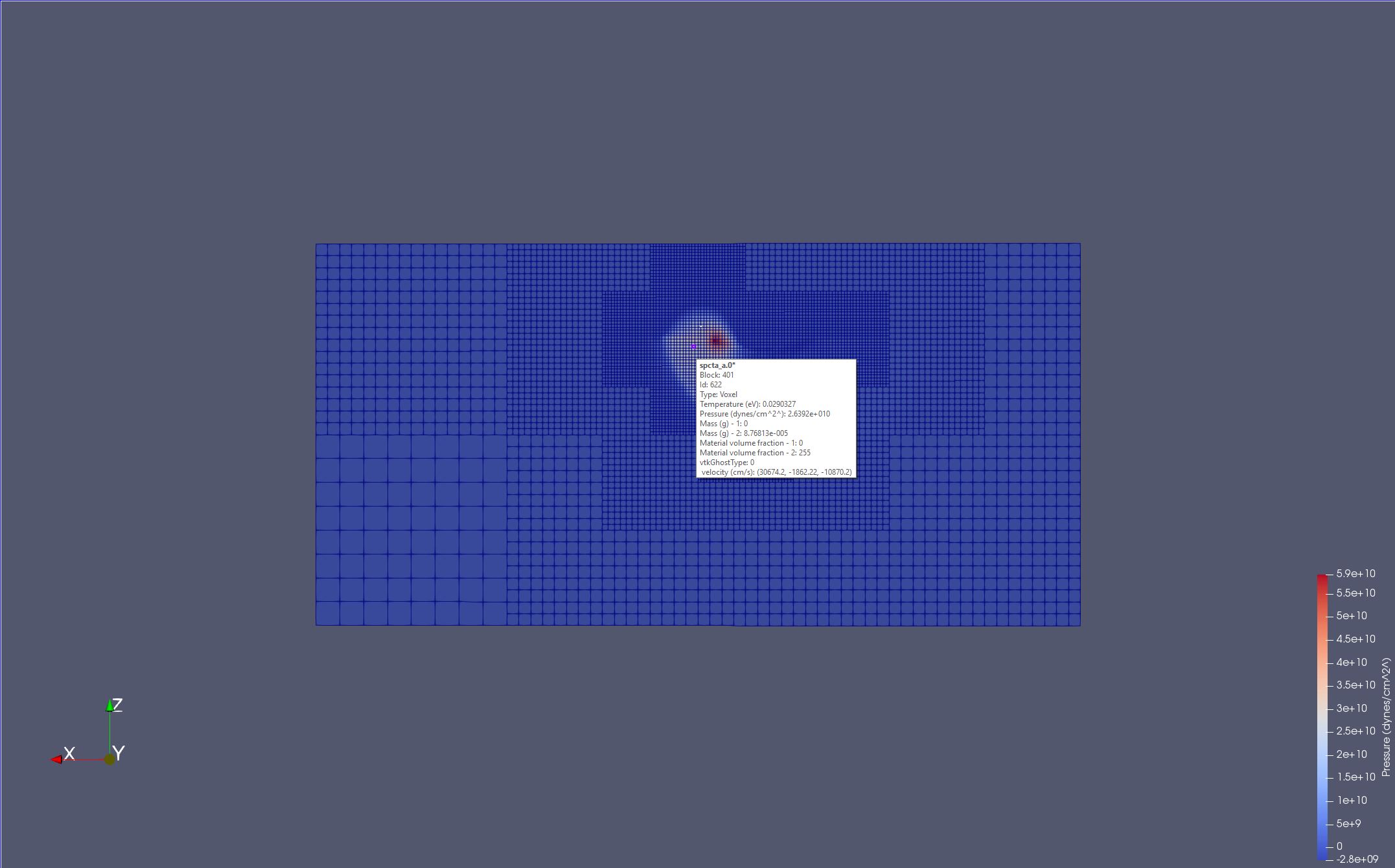
15.6. Showing cell data
Our next goal is to drill into and show individual cells’ data. This is done with the the Hover Cells On function.
Lets start again from scratch.
Edit/Reset Session.
Open spcth_a.0.[0-3].
Turn all variables on.
Apply.
We need a solid surface in which to work.
Representation: Surface with Edges
Set Coloring to Pressure
-Y
Now, click on the Hover Cells On icon, upper left section of the View.
Hover, and stop, over the cells. The cell data will be displayed on screen.
Hover Cells On is the only selection that works, and provides data.
If you want to look at cells in the middle of your dataset, use the Clip, Slice or Clip by Scalar filter to get to your data.
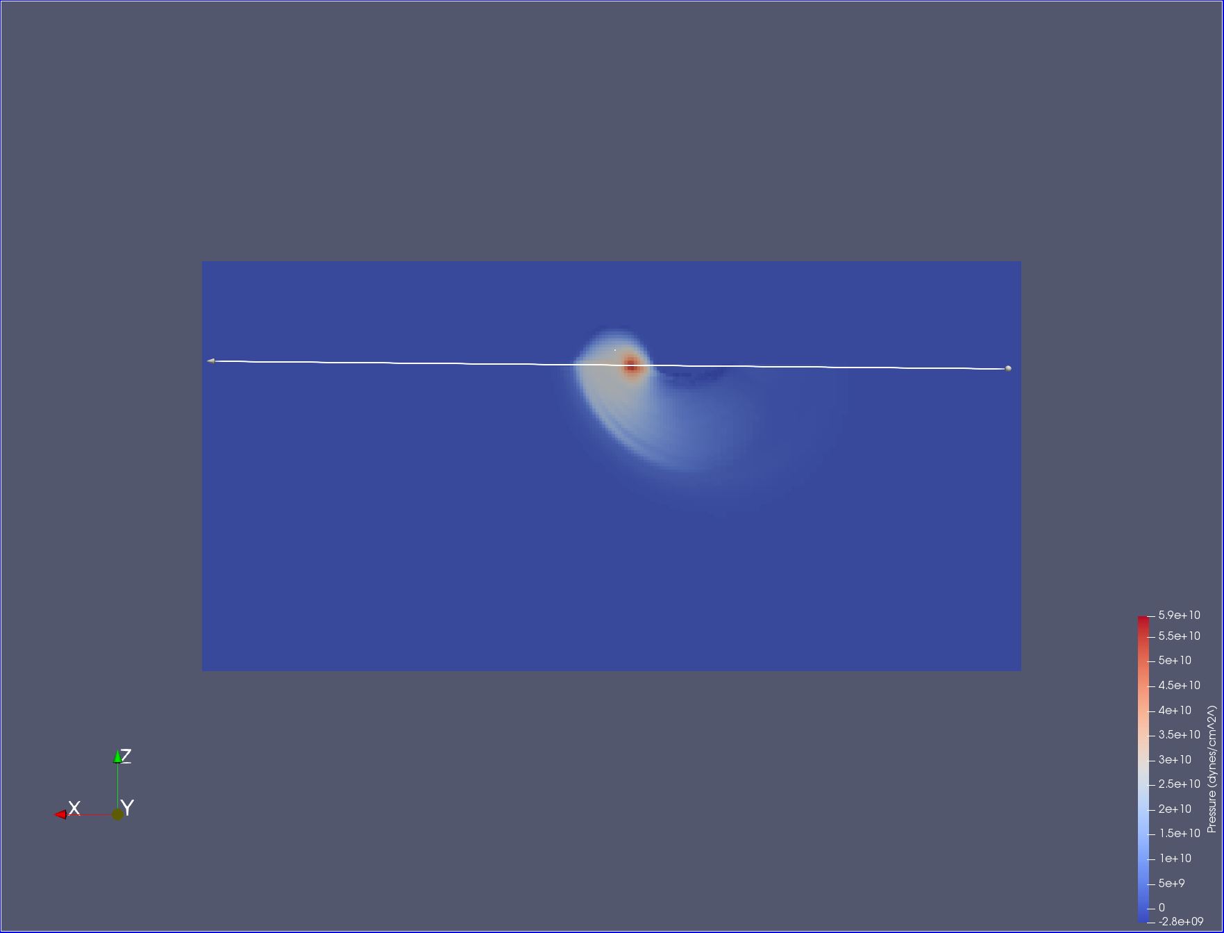
15.7. Plot over line
You can also create a 2d plot along a line through your dataset. Here is how to do it.
Lets start again from scratch.
Edit → Reset Session.
Open spcth_a.0.[0-3].
Turn all variables on.
Apply.
Again, we need a solid surface in which to work.
Set Representation to Surface with Edges.
Set Coloring to Pressure.
-Y.
You can now see where the aluminum ball is hitting the steel block.
Filters → Domain → Data Analysis → Plot Over Line.
Apply.
We want to overlay the line horizontally across the area of interest, just inside of the block. To do this, we will set it on the surface and then move it.
Click X Axis. The line is now horizontal, through your data. The base of the arrow is on the right, the head is to the left.
Place the cursor at the right edge of the block, 3/4 of the way to the top. Hit the 1 key. You have now moved the base.
Place the cursor at the left edge of the block, 3/4 of the way to the top. Hit the 2 key. You have now moved the head.
Make sure the Plot Over Line filter is still selected.
Apply.
In the Properties tab, un-select all variables that you don’t want to plot.

More details on how to run Plot filters can be found in Section 5 of Tutorials.
15.8. Calculating density
Density is calculated in the CTH reader for rectilinear grids, but not for AMR. Here is how to calculate it for AMR grids.
Lets start again from scratch.
Edit → Reset Session.
Open spcth_a.0.[0-3].
Turn all variables on.
Since we need cell volume fraction going from 0 to 1, unselect Down Convert Volume Fraction.
Apply.
Now, we calculate the volume of each cell.
Cell Size.
Only keep Compute Volume checked.
Apply.
Now, we calculate the density.
Select Filters → Common → Calculator.
Set Attribute Type to Cell Data.
Result Array Density.
Set Expression to (Mass(g) – 2) / (Volume *(Material Volume Fraction – 2)).
The goal is divide the mass in a cell by the volume of that cell that is of this material.
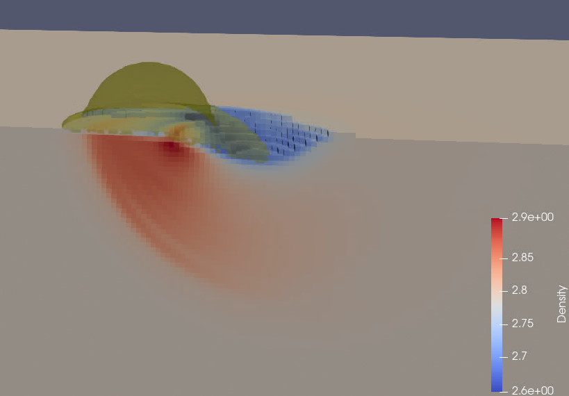
Fig. 15.7 Ball sliding across aluminum plate. Ball is yellow, plate is painted by Density, showing density changes.