2. Beginning: Sources & Filters
2.1. Introduction
This usecase shows a user how to use sources and filters to modify the display of data.
Most examples assume that the user starts with a new model. To start over, go to the menu item Edit → Reset Session, and then re-open your data.
Data is opened by going to File → Open. Example data files can be found in the Examples directory, located in the upper left of the Open dialog.
2.2. Annotate Time Source
Open can.ex2.
Apply.
Drag the can around with the left mouse button until you can see the can.
Select Sources → Annotate Time.
Apply.
Play the animation

2.3. Text Source
This exercise continues on from the previous one. If you are starting over:
Open can.ex2.
Apply.
Select Sources → Text.
Type some text in the window.
Apply.
We now want to move the Text away from the Annotate Time.
In the Properties tab under Text Position are six location icons. Click the Top Center one.
You can manually move the text. Enable this functionality by selecting Use Coordinates, and then moving the text with the mouse.

2.4. Ruler Source
This exercise continues on from the previous one. If you are starting over:
Open can.ex2.
Apply.
Rotate the can so you can see the concave surface.
Select Sources → Ruler.
As noted in the Properties tab, 1 and 2 set the starting and ending points of the ruler onto the can.
Apply.
Did you know?
The line widget has a start and an end. The starting point is marked with a sphere, the ending point is marked with a cone.
Did you know?
If you turn on Auto Apply (see Section 3), you can interactively update the end points of the ruler.
Did you know?
You can use the X, Y or Z key and the mouse to move end points in only one axis.

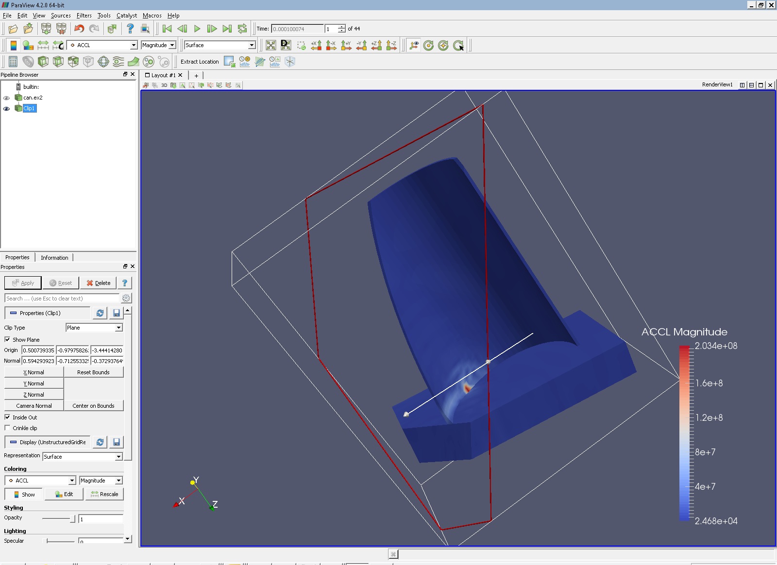
2.5. Clip filter
Open can.ex2.
Apply.
Drag the can around with the left mouse button until you can see the can.
Select Filters → Common → Clip (Notice that this is also the third icon from the top on the far left of the screen.)
Apply.
Press X Normal.
Apply.
Try also Y Normal.
Apply.
Grab the arrow control at the end of the clip object with the left mouse button. Drag it around. You can also grab the red box and slide the clip plane forward and backward.
Apply.
Turn off the Show Plane checkbox.
Select Inside Out.
If the clip arrow control is ever hidden behind data, you can see it by clicking on the “eye” to the left of the “clip” in the Pipeline Browser which is located in upper left corner of the screen.
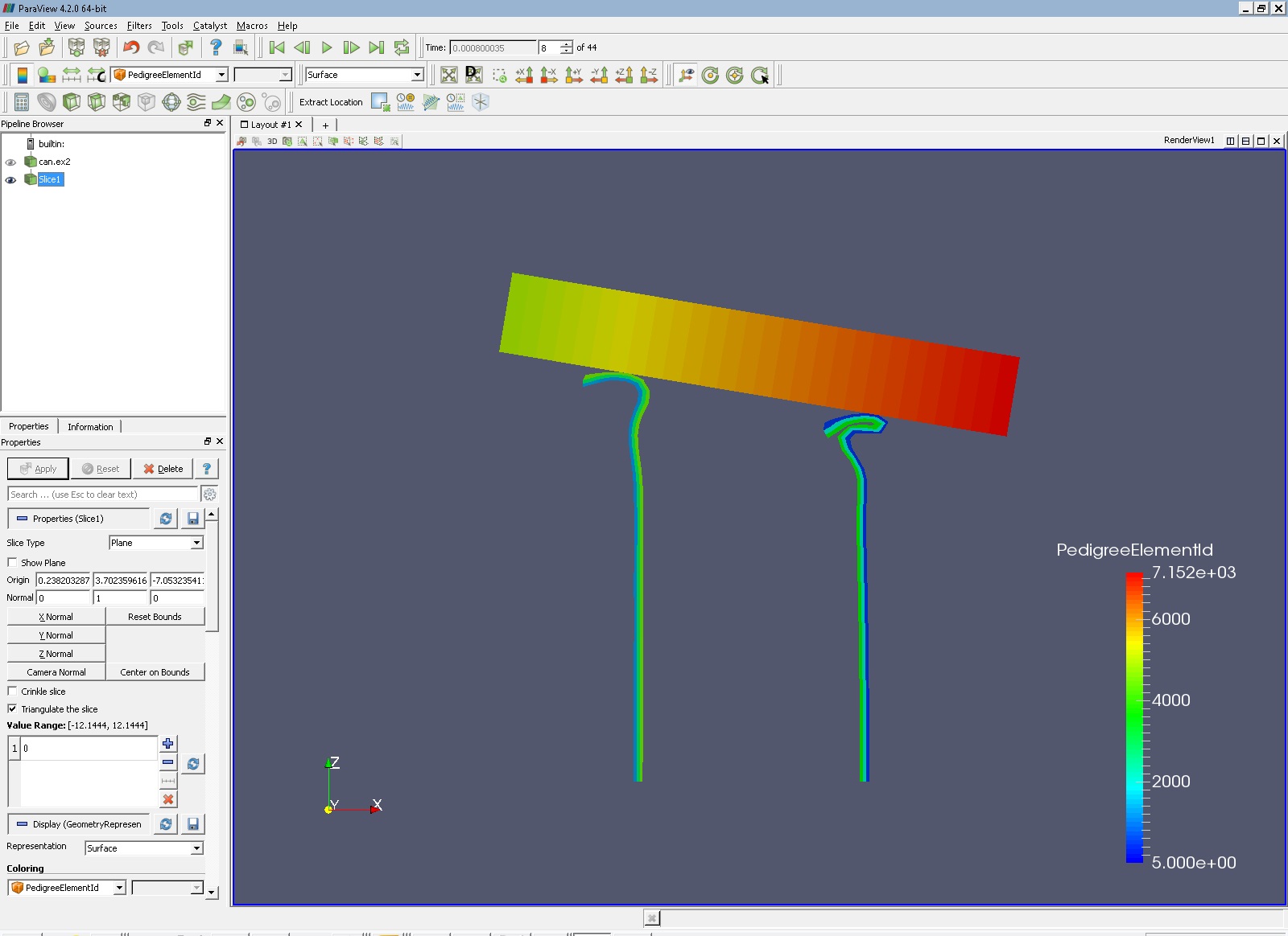
2.6. Slice filter
Open can.ex2.
Apply.
Drag the can around with the left mouse button until you can see the can.
Select Filters → Common → Slice.
Apply.
Press Y Normal.
Apply.
Try also Z Normal.
Apply.
Grab the arrow control at the end of the clip object with the left mouse button. Drag it around.
Apply.
Turn off the Show Plane checkbox.
We need to go to the Advanced Properties tab. Click on the little gear to the right of the search box.
In the Slice Offset Value section, press New Value, type 1. Apply. Notice that we just added a second cut plane.
Under Slice Offset Values, press Delete All. Select New Range. Input From value of -4 and To value of 4. OK. Apply. Now we have 10 slices through our object.
Play the animation.
If the slice arrow control is ever hidden behind data, you can see it by clicking on the “eye” to the left of the “clip” in the Pipeline Browser which is located in upper left corner of the screen.
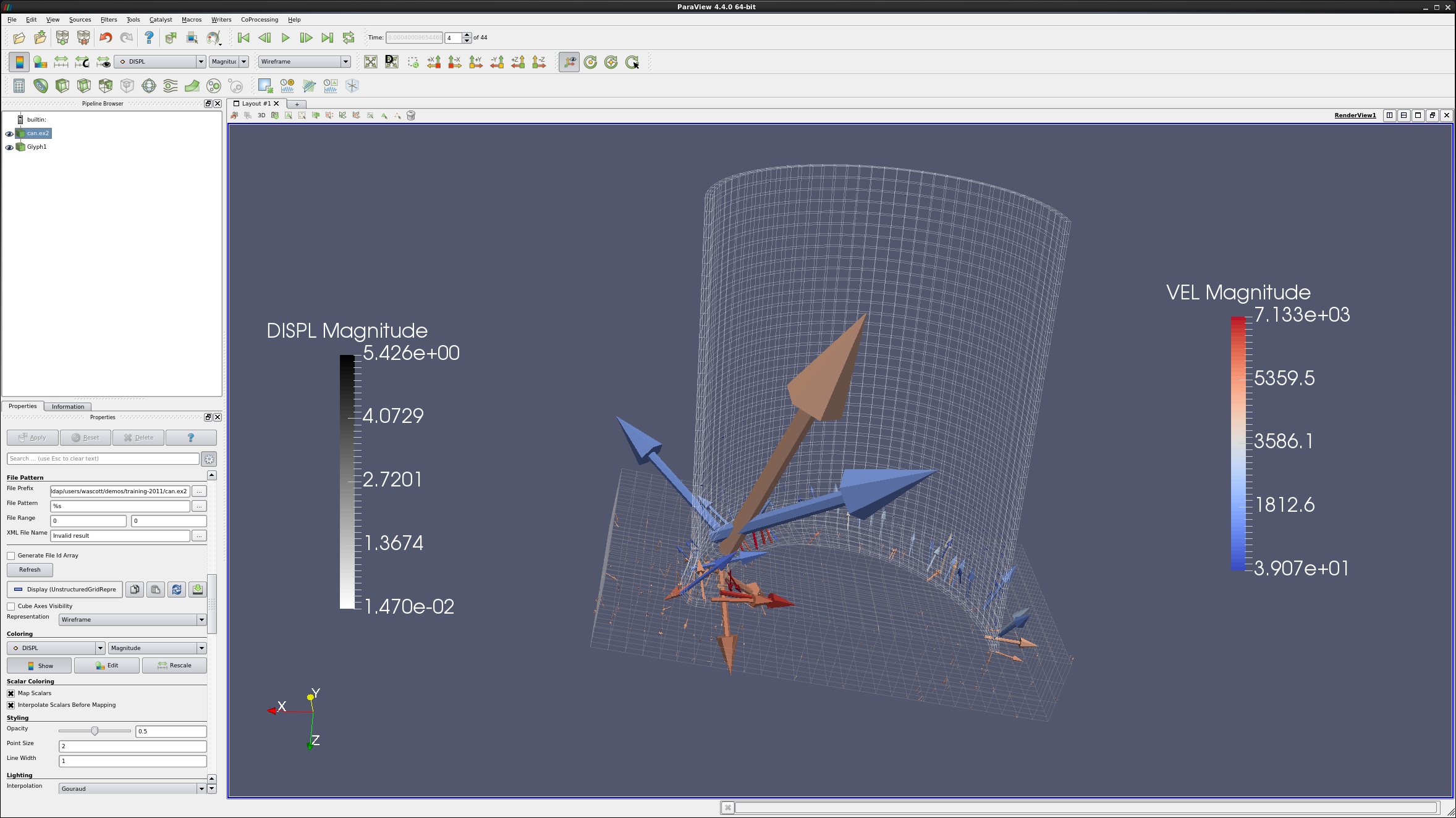
2.7. Glyph filter
Open can.ex2.
Apply.
Drag the can around with the right mouse button until you can see the can.
Select Filters → Common → Glyph.
Change the Vectors to ACCL.
Apply.
paraviewdoes not set the Scale Factor correctly. On the Properties tab is an entry for Set Scale Factor. Change this to 1e-7.Apply.
Click the Play button at the top of the screen.
Reset by hitting the First Frame button.
We want to see the glyphs in context. Turn the visibility eyeball on the can.ex2 to “on”.
Click on can.ex2 (it will show up as blue).
In the Properties tab, Set Representation → Wireframe.
Play the animation. We can now see where the accelerations are occurring as the can is crushed.
Reset the animation.
Click on the Glyph in the Pipeline Browser, thus giving the Glyph focus.
In the Properties tab, change the Vectors to VEL.
Then, change the Set Scale Factor to 3e-4.
Apply.
Re-animate the window.
Extra credit – Change the color of the glyphs to match the picture below.
2.8. Threshold filter
Open disk_out_ref.ex2.
Apply.
Spin the object around, and look inside of it.
Press the Threshold button , found to the far left. (Notice that you can also find this through the filters menu.)
Select Scalars “Temp” (Temperature).
Note: The blue recycle button will set the min and max values.
Change the Lower Threshold to 400.
Apply.
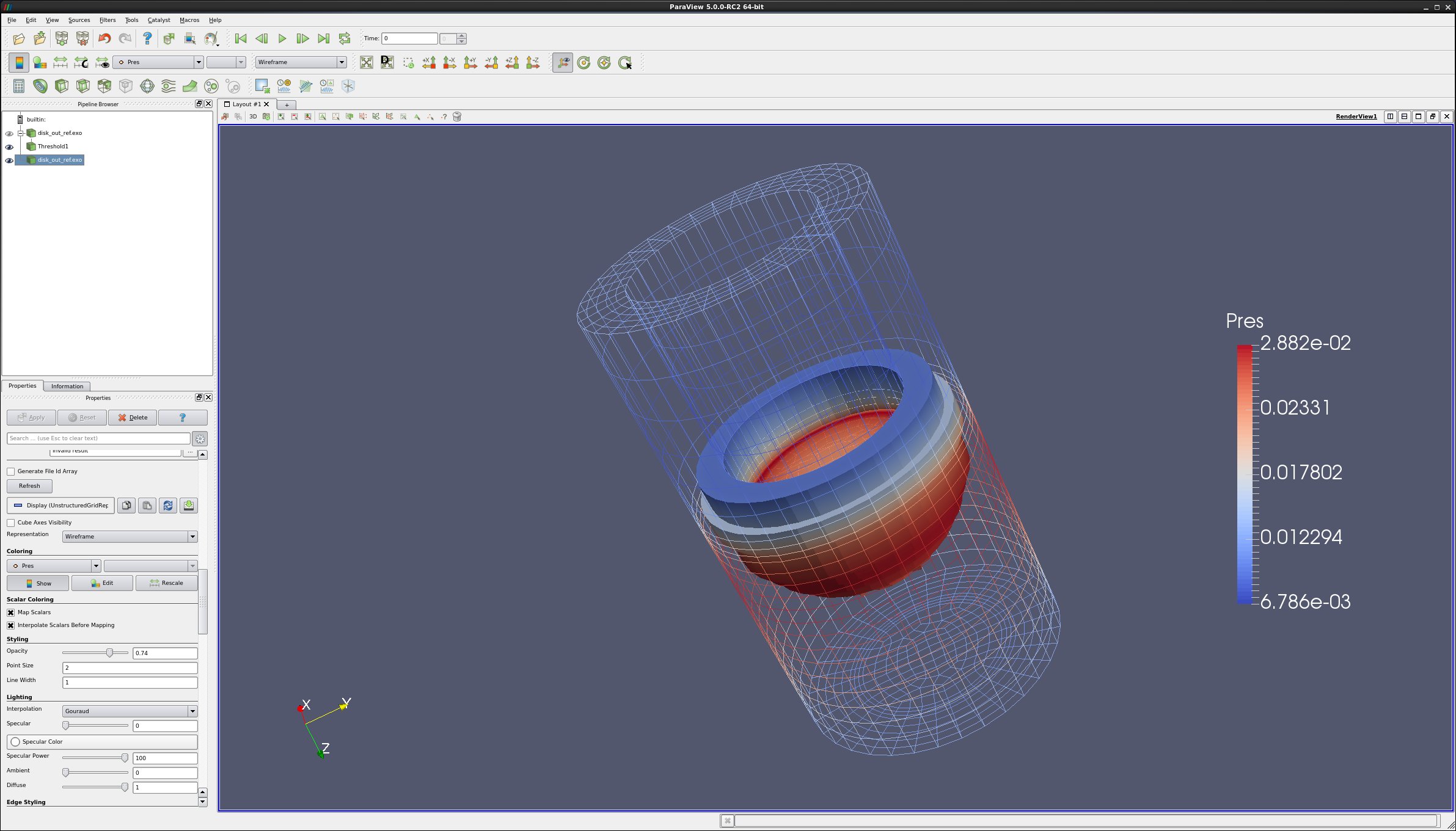
Set Coloring to Pres.
Spin the object around, and look at it.
Now, let’s place this hot section back into the cylinder.
Let’s open another version of disk_out_ref.ex2, using the File → Open menu.
Apply.
Make sure that the second disk_out_ref.ex2 is highlighted in the Pipeline Browser
Set Representation to Wireframe.
In the Properties tab, set Coloring to Pres
What we have done: We have created an unstructured grid holding the cells that fit our criteria. This can make our data much bigger, and should be avoided if we are working with big data.
Extra credit:
Change the outside cylinder to be volume rendered, set Representation to Volume.
2.9. Contour filter
Open disk_out_ref.ex2.
Apply.
Select Filters → Common → Contour.
Change Properties: Contour By: to Temp.
Under Value Range, press Delete All.
Now press New Value and enter 400.
Apply.
Set Coloring to Temp.
Why are all parts of the object the same color?
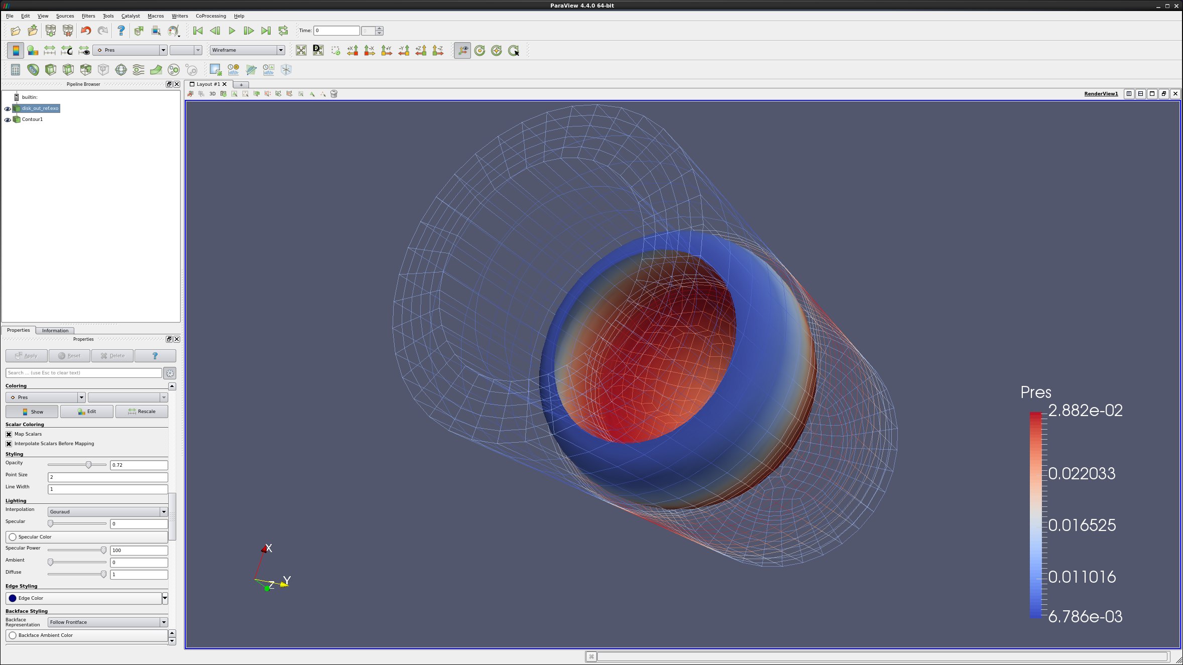
Set Coloring to Pres (Pressure).
This represents the location inside of the cylinder that is at temperature 400, and is colored by pressure.
Turn the visibility back on for the disk_out_ref.ex2.
In the Pipeline Browser, click disk_out_ref.ex2 (turning it white)
Select Representation Wireframe.
Set Coloring to Pres.
Notice that this is another way to see two representations of the same object by reading the object in once and modifying it. In the Threshold Filter (above), we read in the object twice, and displayed each object differently.
What we have done: We have created an isosurface of a specific temperature. One nice thing about isosurfaces is that they decrease the amount of data that has to fit into memory. This is handy when you are displaying big data.
Extra credit:
Highlight disk_out_ref.ex2.
Select Clip filter.
Select X Normal for the clip plane. - Why has the disk_out_ref.ex2 model now turned solid? (Hint – the visibility has changed)
More extra credit:
Under contour, Advanced Properties tab, delete the Isosurface, and use New Range to create 10 new surfaces. Again, the Advanced Properties tab is enabled by clicking on the gear icon to the right of the search box.
Next, select Clip filter to cut the cylinder in half.
What are the surfaces showing us? What are the colors showing us?
Highlighting clip
Under Properties tab, change the Opacity to .50.
2.10. Clip to Scalar filter
Open disk_out_ref.ex2.
Apply.
Select Filters → Recent → Clip.
Apply.
Select Clip Type → Scalar.
Select Scalars → Temp.
Input a Value of 400.
Apply.
Select Clip filter again.
Unclick Show Plane.
Apply.
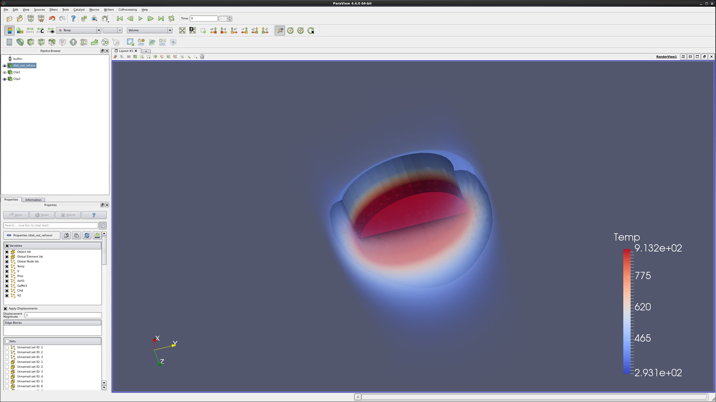
Set Coloring to Temp.
Highlight disk_out_ref.ex2, turn the eyeball on.
Display by Volume
Set Coloring to Temp.
What we have done: We have clipped to a constant scalar, creating a smooth mesh. Once again, this increases the size of your data significantly.
2.11. Cell to Point/ Point to Cell filters
These filters are used to convert a dataset from having cell data to having point data and vice versa. This is sometimes useful if a filter requires one type of data, and a user only has the other type of data. An example would be using can.ex2. You cannot get a contour of EQPS directly, since EQPS is cell data and contour only works on points. Use the filter Cell Data to Point Data first, then call contour.
2.12. Stream Tracer
Open disk_out_ref.ex2.
Apply.
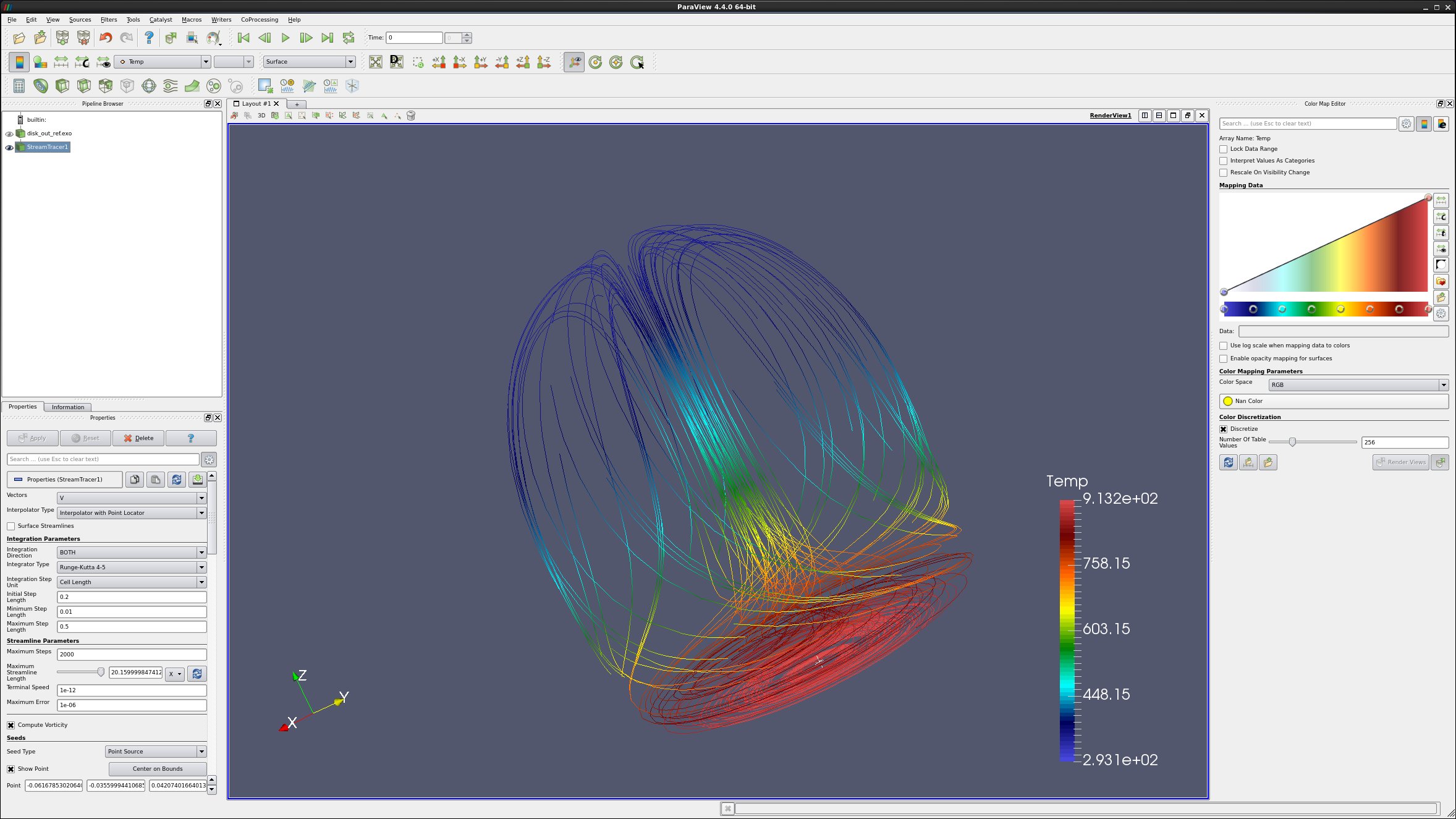
Select Filters → Common → Stream Tracer.
Click the Seeds: Center on Bounds button.
Apply.
In the Properties tab, set Coloring to Temp, then V, then Pres.
If necessary, click Color, Reset Range.
Extra credit:
On the Properties page, set the Number of Points to 40.
Apply.
Select Filters → Alphabetical → Tube.
Apply.
2.13. Calculator filter
Open disk_out_ref.ex2.
Apply.
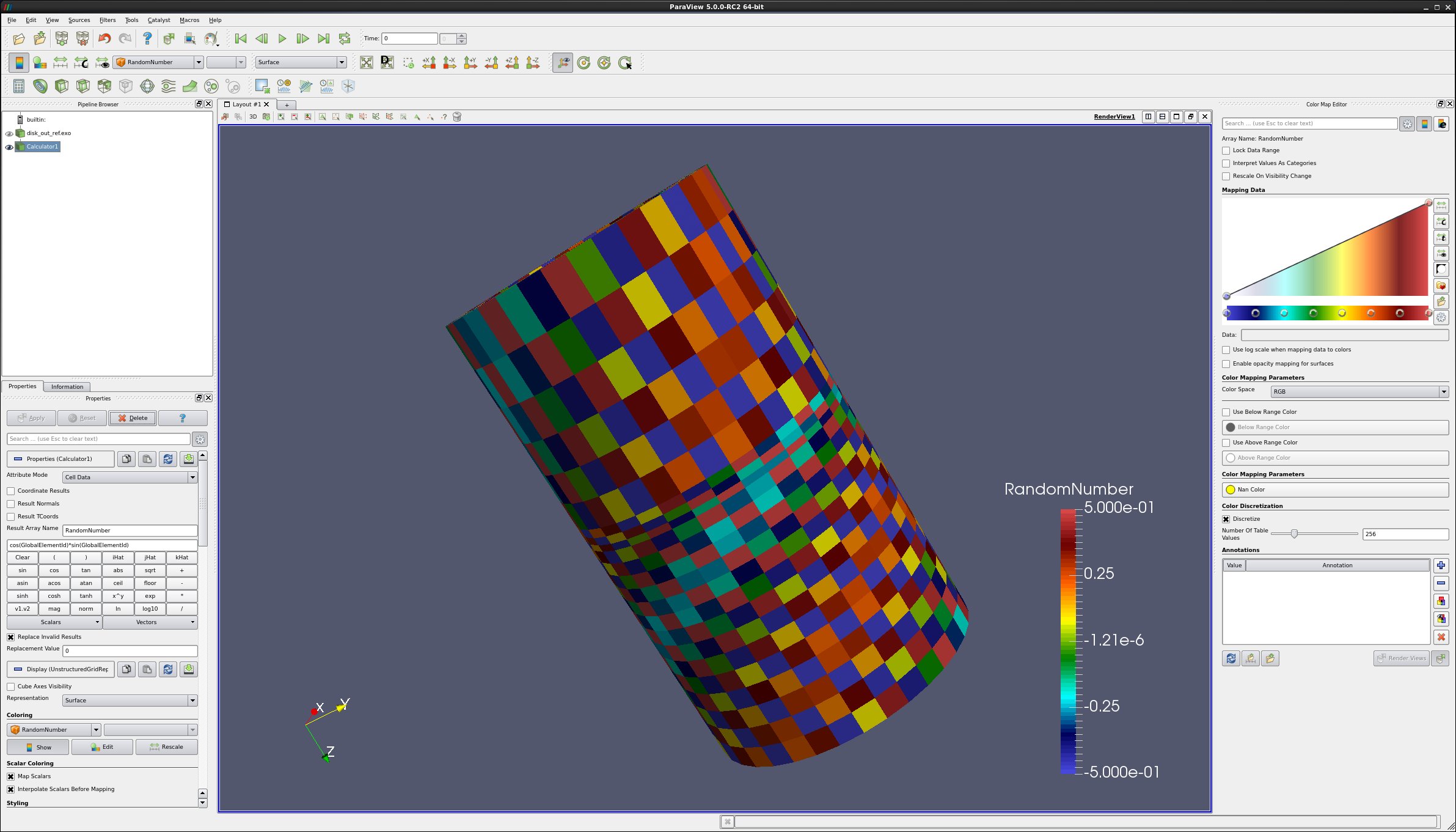
Select Filters → Common → Calculator.
Select Attribute Mode: Cell Data.
Set Result Array Name to RandomNumber.
In the empty line below, type cos(GlobalElementId)*sin(GlobalElementId).
Did you know?
You can pull in the names of the variables by clicking on the Scalars/Vectors button.
In the Properties tab, set Coloring to RandomNumber.
We are now coloring by a pseudo random number. This shows how complex our data is.
Note that you can create a vector from three scalars using the calculator. For instance, to create an X,Y,0 vector from Velocity, type VEL_X*iHat+VEL_Y*jHat+0*kHat.
To get the length of a vector, use mag(vector_name).
To get the length of a vector squared, use mag(vector_name)*mag(vector_name).
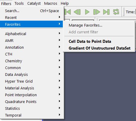
2.14. Favorites
paraview allows users to place their favorite filters into the submenu
named Filters → Favorites. Just use the Manage Favorites tool.
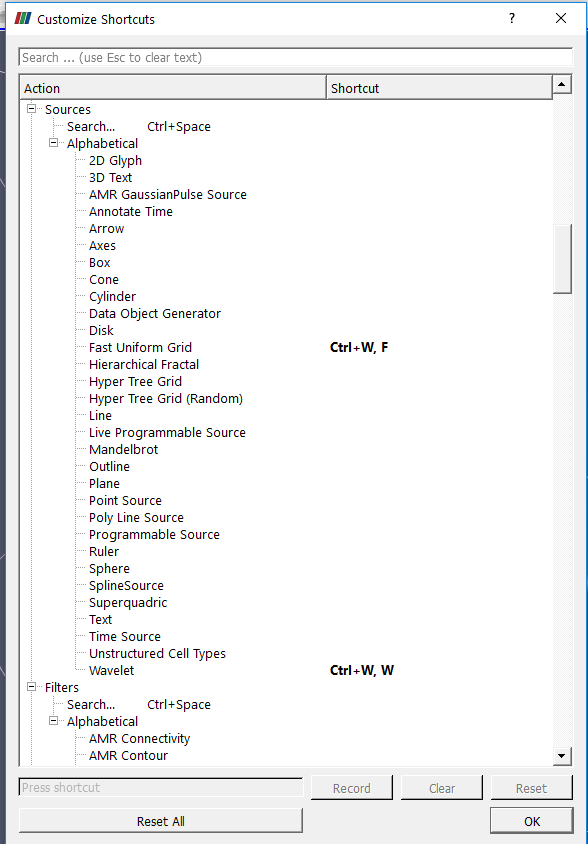
2.15. Customize Shortcuts
paraview allows users to add keyboard shortcuts to your favorite menu or
filter. This is found under Tools → Customize Shortcuts.