11. Advanced: Tips & Tricks
11.1. Introduction
This section holds tips and tricks that don’t fit anywhere else, or are small enough that they don’t deserve their own tutorial.
11.2. Creating a Custom Filter
Open disk_out_ref.ex2.
Apply.
In the Properties tab, Set Coloring to Temp.
Select Clip filter.
Set Clip type to Scalar. (The Scalars and Values don’t matter right now)
Apply.
Select Tools → Create Custom Filter.
Name this filter ClipByScalar (IsoVolume).
Take the default inputs.
Take the default outputs.
Select the clip (in the left window), and pull down the pull down menu for Property.
Select Scalars.
Hit the blue + sign.
Do the same for Value and Inside Out.
Finish.
Now, delete the Clip filter in the pipeline browser.
Select Filters → Alphabetical → ClipByScalar (sometimes incorrectly know as an IsoVolume filter).
Turn Scalars to Temp
Enter a Value of 400.
Apply.
11.3. Temporal Statistics Filter
Open can.ex2.
Apply.
Filters → Temporal → Temporal Statistics.
Apply.
Set Coloring to ACCL_average.
Set Coloring to ACCL_maximum.
Set Coloring to DISPL_average.
You can now visually see average acceleration, maximum acceleration and average displacement of each cell.
To see the ranges of these variables over the whole mesh, look in the Information tab.

11.4. Creating vectors from 2 or 3 scalars
See Calculator in the tutorial Beginning Sources and Filters
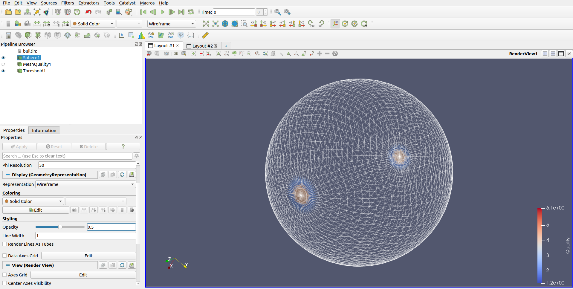
11.5. Mesh quality
Select Sources → Alphabetical → Sphere.
In the Properties tab, set Theta Resolution and Phi Resolution to 50.
Apply.
Select Filters → Alphabetical → Mesh Quality. and use defaults.
Apply.
Next, we want to only look at those cells that are below some threshold of quality.
Filters → Common → Threshold.
Choose Scalars of “Quality”, and Lower Threshold of 2.3 and Upper Threshold of 10.
Turn visibility of Sphere1 on.
Set Representation → Wireframe.
Set Opacity to 0.5.

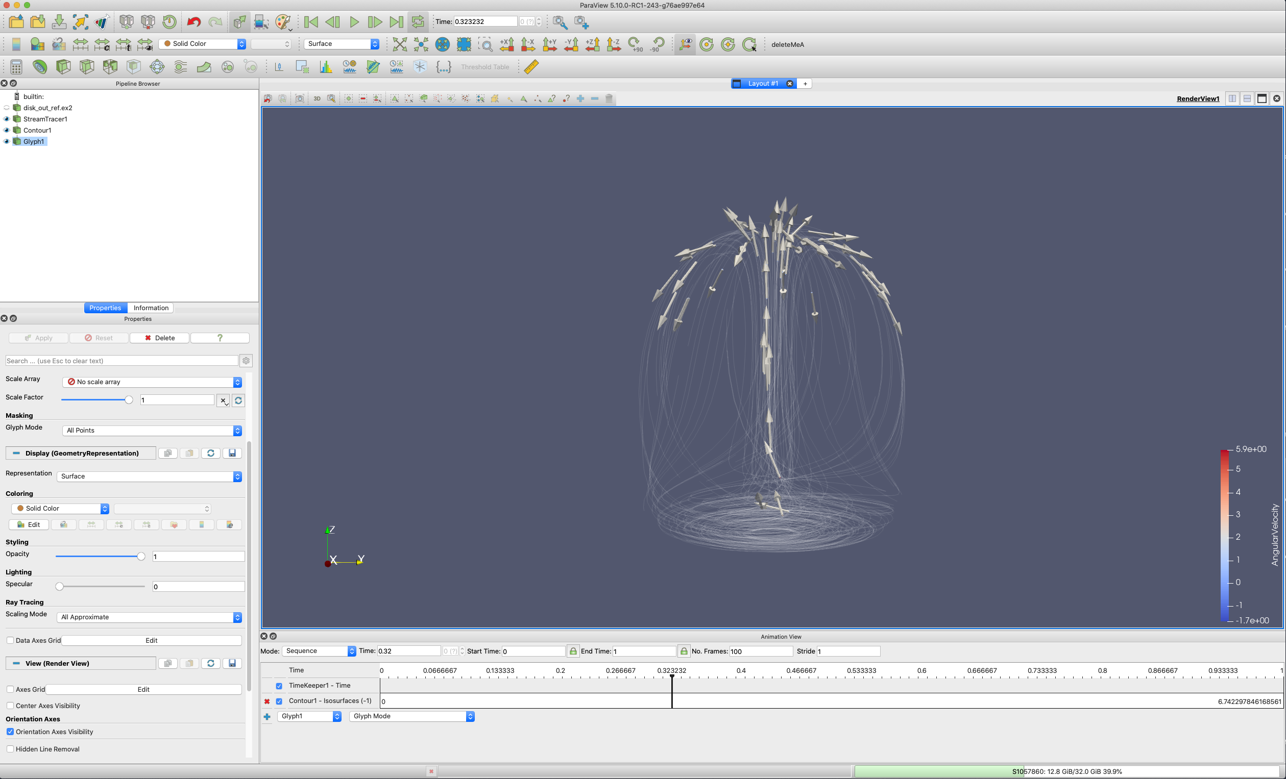
11.7. Animating a static vector field
If you have a vector field in your data, you can animate a static dataset.
Our goal is to create a set of streamlines from a vector field, place points on this set of streamlines, and animate the point down the streamlines. We will also add glyphs to the streamline points.
Open disk_out_ref.ex2.
Apply.
Click -X.
Select Filters → Common → Stream tracer. (We are already streamtracing on V).
Set Seed Type to Point Cloud.
Unckeck Show sphere.
Set Opacity to 0.3.
Apply.
Open View → Color Map Editor.
Click Invert the transfer functions.
Select Filters → Common → Contour.
Contour on IntegrationTime.
Apply.
Select Filters → Common → Glyph.
Set Orientation Array to v.
Set Glyph Mode to All Points.
Set Scale factor to 0.5.
Set Coloring to v.
Apply.
In the Pipeline browser, hide Contour1, and show SteamTracer1 and Contour1.
View → Animation View.
Set Mode to Sequence.
Set No. Frames to 100.
Change the pulldown box next to the blue + to be Contour1.
Click the blue +.
Play.