4. Visualizing Large Models
ParaView is used frequently at Sandia National Laboratories and other institutions for visualizing data from large-scale simulations run on the world’s largest supercomputers including the examples shown here.
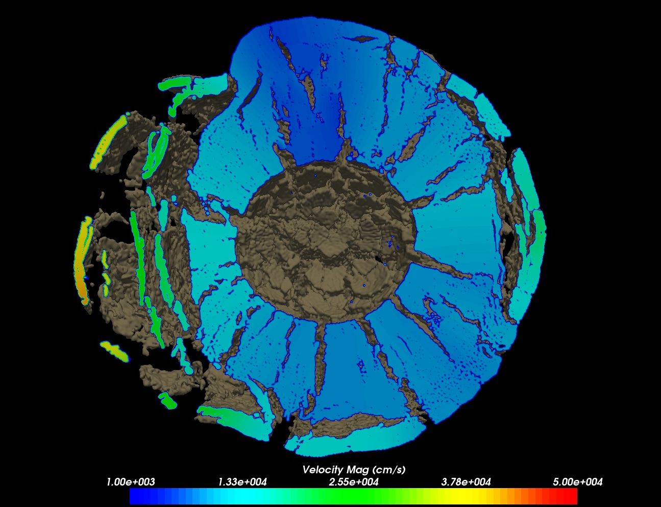
Fig. 4.43 CTH shock physics simulation with over 1 billion cells of a 10 megaton explosion detonated at the center of the Golevka asteroid.
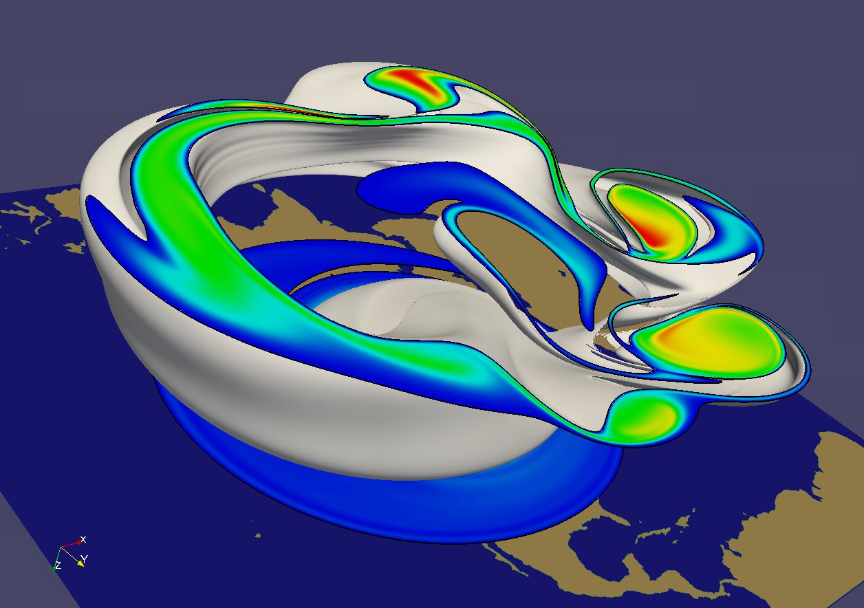
Fig. 4.44 SEAM Climate Modeling simulation with 1 billion cells modeling the breakdown of the polar vortex, a circumpolar jet that traps polar air at high latitudes.
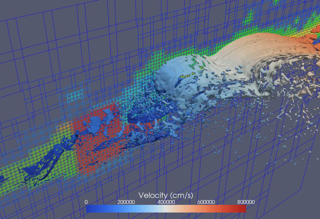
Fig. 4.45 A CTH simulation that generates AMR data. ParaView has been used to visualize CTH simulation AMR data comprising billions of cells, 100’s of thousands of blocks, and eleven levels of hierarchy (not shown).
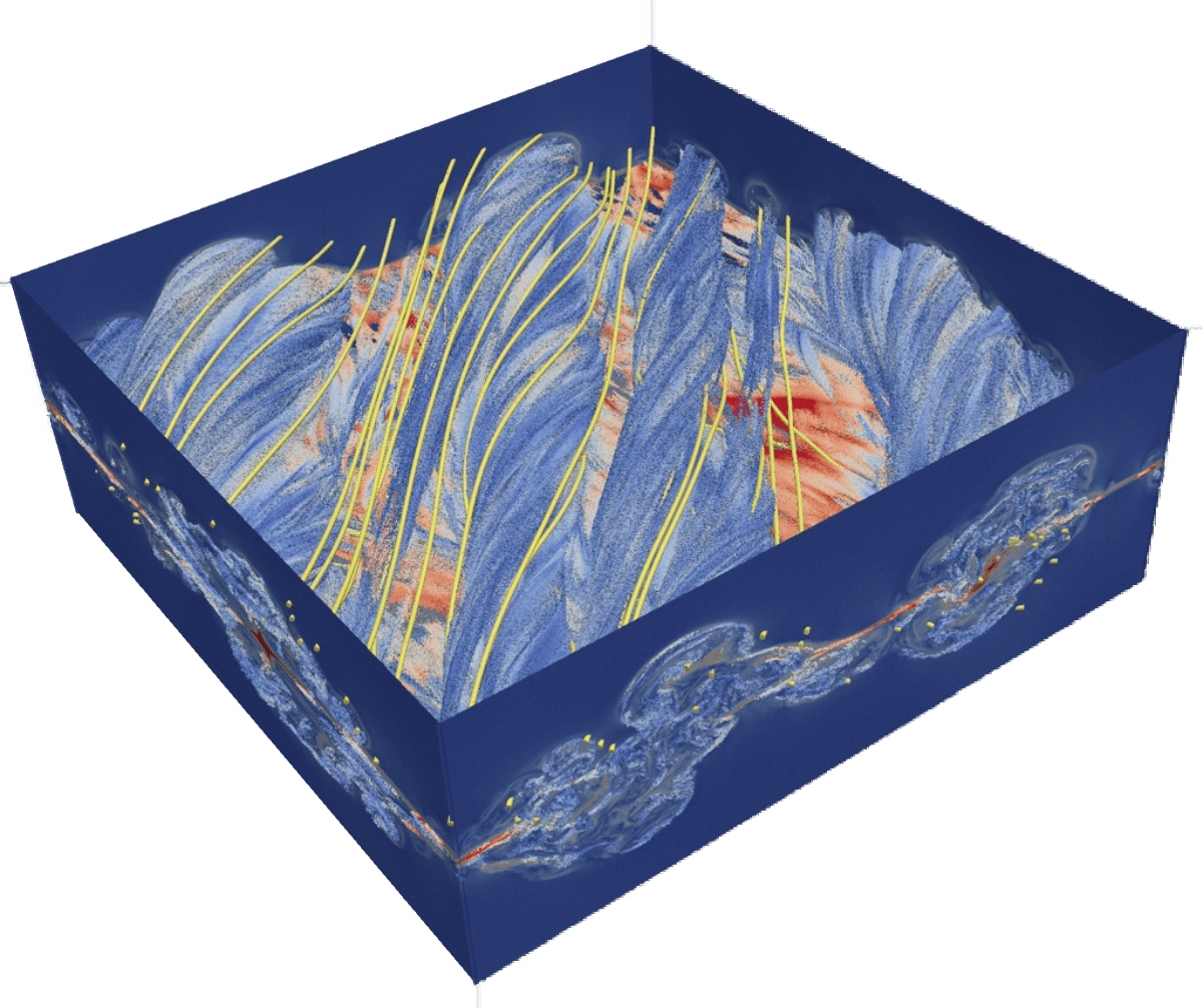
Fig. 4.46 A VPIC simulation of magnetic reconnection with 3.3 billion structured cells. Image courtesy of Bill Daughton, Los Alamos National Laboratory.
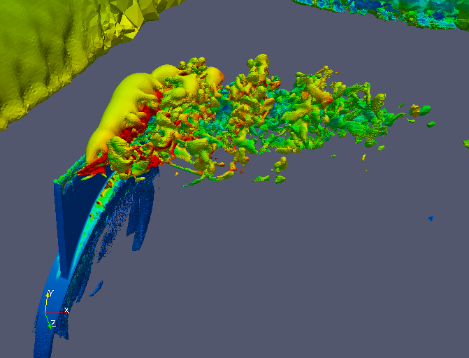
Fig. 4.47 A large scale in-situ PHASTA simulation that generated a 3.3 billion tetrahedral mesh simulating the flow over a full wing where a synthetic jet issues an unsteady crossflow jet (run on 160 thousand MPI processes).
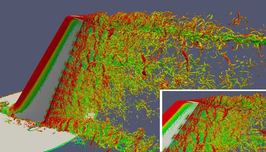
Fig. 4.48 A large scale in-situ PHASTA simulation that generated a 1.3 billion element mesh simulating the wake of a deflected wing flap (run on 256 thousand MPI processes). Images courtesy of Michel Rasquin, Argonne National Laboratory.
In this section we discuss visualizing large meshes like these using the parallel visualization capabilities of ParaView. This section has some exercises, but is less “hands-on” than the previous section. Primarily you will learn the conceptual knowledge needed to perform large parallel visualization. The exercises demonstrate the basic techniques needed to run ParaView on parallel machines.
The most fundamental idea to grasp is that when run on a large machine every node processes different regions of the entire dataset simultaneously. Thus the workable data resolution is limited by the aggregate memory space of the machine. We now present the basic ParaView architecture and parallel algorithms and demonstrate how to apply this knowledge.
4.1. Parallel Visualization Algorithms
We are fortunate in visualization in that many operations are straightforward to parallelize. The data we deal with is contained in a mesh, which means the data is already broken into little pieces by the cells. We can do visualization on a distributed parallel machine by first dividing the cells among the processes. For demonstrative purposes, consider this very simplified mesh.

Now let us say we want to perform visualizations on this mesh using three processes. We can divide the cells of the mesh as shown below with the blue, yellow, and pink regions.
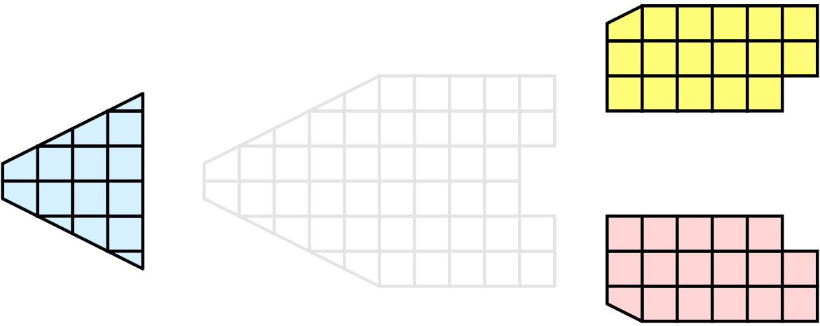
Once partitioned, many visualization algorithms will work by simply allowing each process to independently run the algorithm on its local collection of cells. For example, take clipping (which is demonstrated in multiple exercises including Exercise 2.11). Let us say that we define a clipping plane and give that same plane to each of the processes.
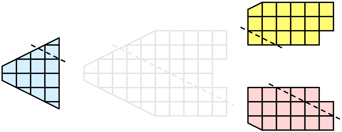
Each process can independently clip its cells with this plane. The end result is the same as if we had done the clipping serially. If we were to bring the cells together (which we would never actually do for large data for obvious reasons) we would see that the clipping operation took place correctly.

Many, but not all operations are thus trivially parallizeable. Other operations are straightforward to parallelize if ghost layers as described in Section 4.7.2 are available. Other operations require more extensive data sharing among nodes. In these filters ParaView resorts to MPI to communicate amongst the nodes of the machine.
4.2. Basic Parallel Rendering
When performing parallel visualization, we are careful to ensure that the data remains partitioned among all of the processes up to and including the rendering processes. ParaView uses a parallel rendering library called IceT. IceT uses a sort-last algorithm for parallel rendering. This parallel rendering algorithm has each process independently render its partition of the geometry and then composites the partial images together to form the final image.
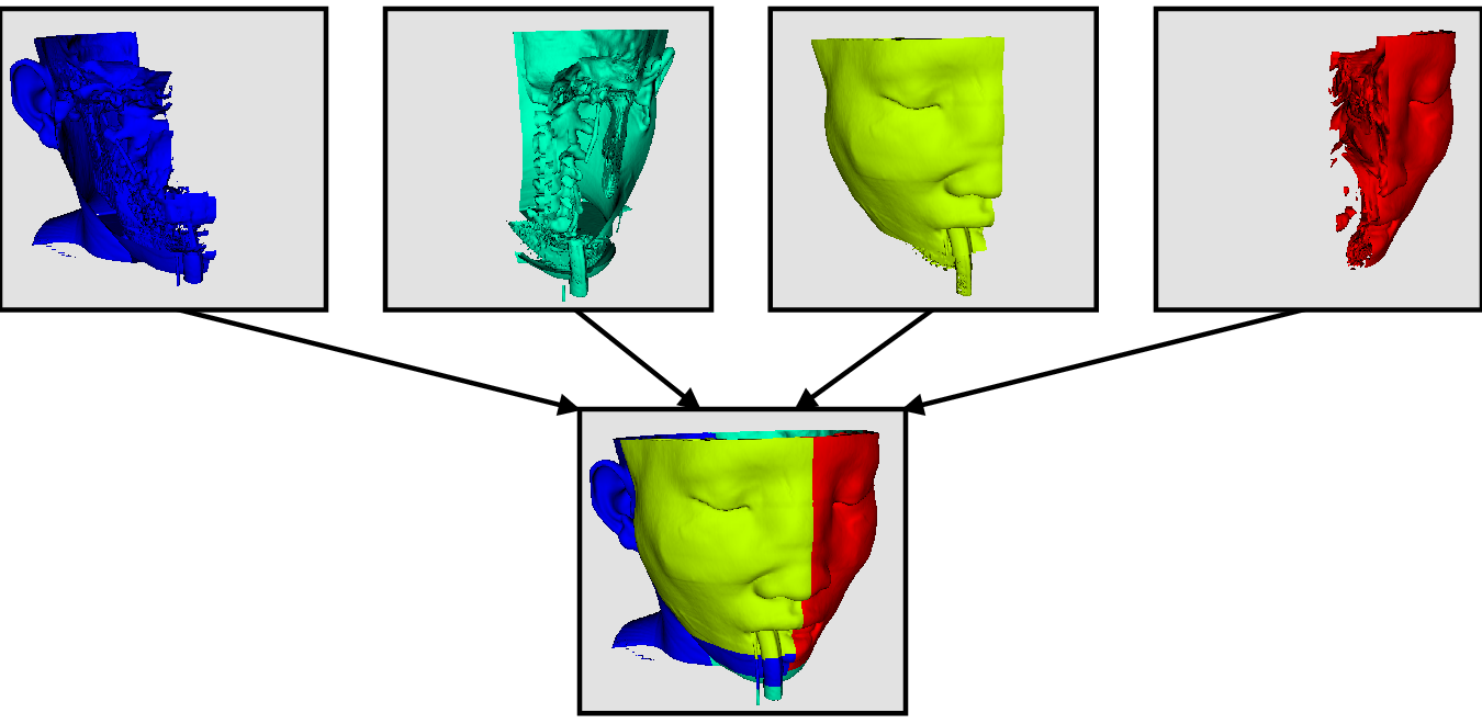
The preceding diagram is an oversimplification. IceT contains multiple parallel image compositing algorithms such as binary tree, binary swap, and radix-k that efficiently divide work among processes using multiple phases.
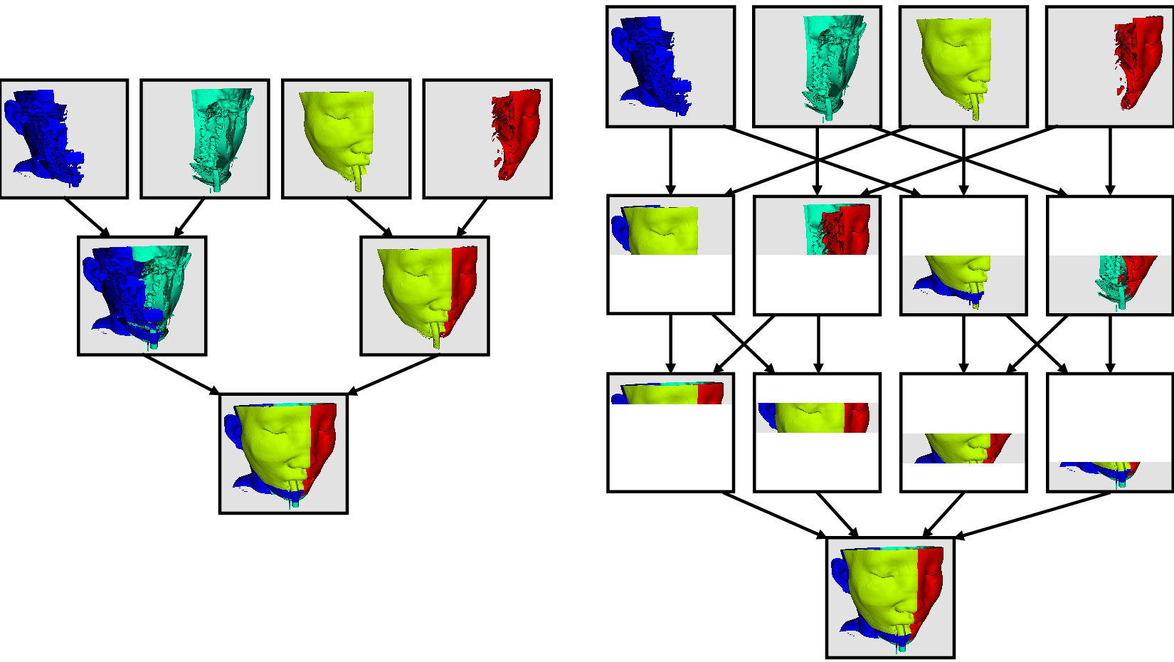
The wonderful thing about sort-last parallel rendering is that its efficiency is completely insensitive to the amount of data being rendered. This makes it a very scalable algorithm and well suited to large data. However, the parallel rendering overhead does increase linearly with the number of pixels in the image. This can be a problem for example when driving tile display walls with ParaView. Consequently, some of the rendering parameters described later in this chapter deal with limiting image size.
Because there is an overhead associated with parallel rendering, ParaView can also render serially and will do so automatically when the visible data is small enough. When the visible meshes are smaller than a user defined threshold preference, or when parallel rendering is turned off or unavailable, the geometry is shipped to the display node, which then rasterizes it locally. Obviously, this should only happen when the data being rendered is small or the rendering process will be overwhelmed.
4.3. ParaView Architecture
With this introduction to parallel visualization, it is useful to know something about how ParaView is structured and how it orchestrates the parallel tasks described above.
ParaView is designed as a three-tier client-server architecture. The three logical units of ParaView are as follows.
- Data Server
The unit responsible for data reading, filtering, and writing. All of the pipeline objects seen in the pipeline browser are contained in the data server. The data server can be parallel.
- Render Server
The unit responsible for rendering. The render server can also be parallel, in which case built in parallel rendering is also enabled.
- Client
The unit responsible for establishing visualization. The client controls the object creation, execution, and destruction in the servers, but does not contain any of the data (thus allowing the servers to scale without bottlenecking on the client). If there is a GUI, that is also in the client. The client is always a serial application.
These logical units need not be physically separated. Logical units are often embedded in the same application, removing the need for any communication between them. There are three modes in which you can run ParaView. Note that no matter what mode ParaView runs in the user interface and scripting API that you learned in Section 2 and Section 3 undergoes very little change.
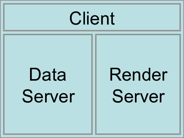
The first mode, which you are already familiar with, is standalone
mode. In standalone mode, the client, data server, and render server are
all combined into a single serial application. When you run the
paraview application, you are automatically connected to a
builtin server so that you are ready to use the full features of
ParaView.
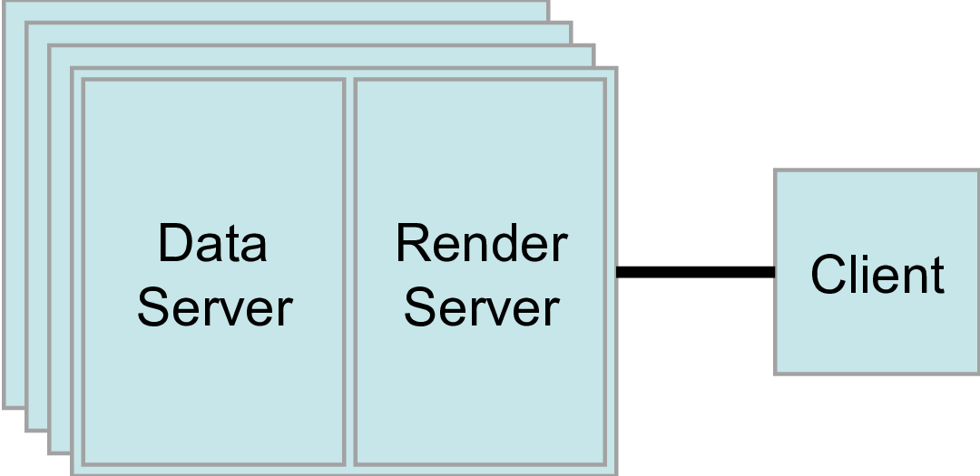
The second mode is client-server mode. In client-server mode, you
execute the pvserver program on a parallel machine and connect to it
with the paraview client application. The pvserver program has
both the data server and render server embedded in it, so both data
processing and rendering take place there. The client and server are
connected via a socket, which is assumed to be a relatively slow mode of
communication, so data transfer over this socket is minimized.
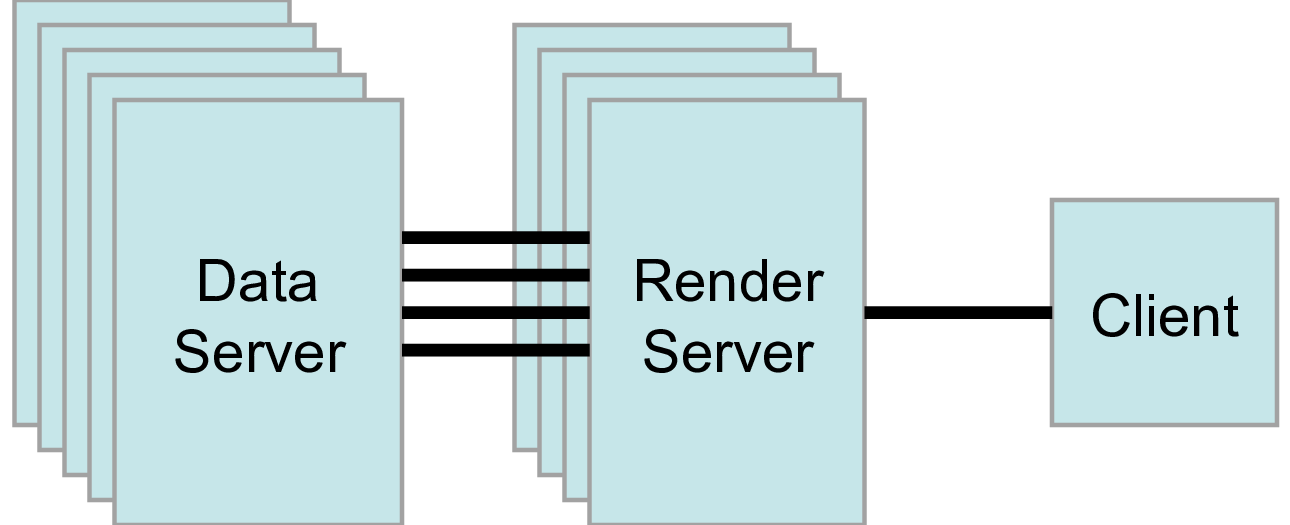
The third mode is client–render-server–data-server mode. In this mode, all three logical units are running in separate programs. As before, the client is connected to the render server via a single socket connection. The render server and data server are connected by many socket connections, one for each process in the render server. Data transfer over the sockets is minimized.
Although the client-render server-data server mode is supported, we almost never recommend using it. The original intent of this mode was to take advantage of heterogeneous environments where one might have a large, powerful computational platform and a second smaller parallel machine with graphics hardware in it. However, in practice we find any benefit is almost always outstripped by the time it takes to move geometry from the data server to the render server. If the computational platform is much bigger than the graphics cluster, then use software rendering on the large computational platform. If the two platforms are about the same size just perform all the computation on the graphics cluster.
4.4. Accessing a Parallel ParaView Server
Accessing a standalone installation of ParaView is trivial. Download and install a pre-compiled binary or get it from your package manager, and go. To visualize extreme scale results, you need to access an installation of ParaView, built with the MPI components enabled, on a machine with sufficient aggregate memory to hold the entire dataset and derived data products. Accessing a parallel enabled installation of ParaView’s server is intrinsically harder than acessing a standalone version.
Recent binary distributions of ParaView provided by Kitware do include MPI for Mac, Linux and optionally Windows. The Windows MPI enabled binaries depend upon Microsoft’s MPI, which must be installed separately. We will not cover those in the rest of this tutorial, but feel free to ask questions on the ParaView mailing list.
Note that the specific MPI library version bundled into the binaries were chosen for widest possible compatibility. For production use ParaView will be much more effective when compiled with an MPI version that is tuned for your machine’s networking fabric. Your system administrators can help you decide what MPI version to use.
To compile ParaView on a parallel machine you or your system administrators will need the following.
CMake cross-platform build setup tool https://www.cmake.org
MPI
OpenGL, either using a GPU in on- (X11) or off- screen (EGL) modes, or in software via Mesa.
Python +NumPy +Matplotlib (all optional but strongly recommended)
Qt \(\ge\) 4.7 (optional)
Compiling without one of the optional libraries means a feature will not be available. Compiling without Qt means that you will not have the GUI application and compiling without Python means that you will not have scripting available. NumPy is almost as important as Python itself, and Matplotlib is helpful for numeric text and some types of views and color lookup tables.
To compile ParaView, you first run CMake, which will allow you to set up compilation parameters and point to libraries on your system. This will create the make files that you then use to build ParaView. For more details on building a ParaView server, see the ParaView Wiki.
https://www.paraview.org/Wiki/Setting_up_a_ParaView_Server#Compiling
Compiling ParaView on exotic machines, for example HPC class machines that require cross compilation and some cloud-based on demand systems, can be an arduous task. You are welcome to seek free advice on the ParaView mailing list or contracted assistance from Kitware.
Fortunately there are a number of large scale systems on which ParaView has already been installed. If you are fortunate enough to have an account on one of these systems, you shouldn’t need to compile anything. The ParaView community maintains an opt in list of these with pointers to system specific documentation on the ParaView Wiki. We invite system maintainers to add to the list if they are permitted to.
https://www.paraview.org/Wiki/ParaView/HPC_Installations
Running ParaView in parallel is also intrinsically more difficult than running the standalone client. It typically involves a number of steps that change depending on the hardware you are running on: logging in to remote computers, allocating parallel nodes, launching a parallel program, and sometimes tunneling through firewalls to establish interactive connections to the compute nodes. These steps are discussed in more detail in the next two sections in which we finally return from theory to practical exercises.
4.5. Batch Processing
ParaView’s Python scripted interface, introduced in Section 3 has the important qualities of being runnable offline, with the human removed from the loop, and being inherently reproducible.
On large scale systems there are two steps that you need to master. The first is to run ParaView in parallel through MPI. The second is to submit a job through the system’s queuing system. For both steps the syntax varies from machine to machine and you should consult your system’s documentation for the details.
We demonstrate how to run ParaView in parallel with the simplest case of running Kitware’s binary in parallel on the PC class system that you have at hand.
Exercise 4.1 (Running a visualization script in parallel)
You will need three things, the mpiexec program to spawn MPI parallel
programs, the pvbatch executable and a Python script.
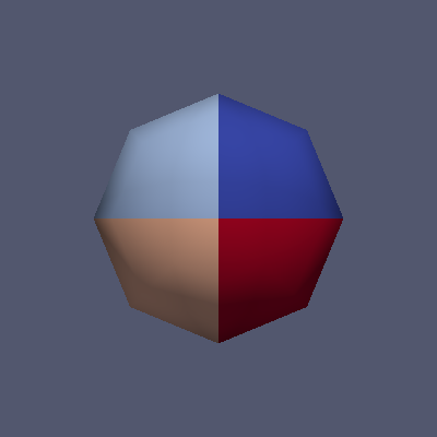
As for the Python script, let us use an example in which each node draws a portion of a simple polygonal sphere with a color map that varies over the number of processes in the job.
from paraview.simple import *
sphere = Sphere()
rep = Show()
ColorBy(rep, ("POINTS", "vtkProcessId"))
Render()
rep.RescaleTransferFunctionToDataRange(True)
Render()
WriteImage("parasphere.png")
Use an editor to type this script into a file called parasphere.py and save it somewhere. Note this is a stripped down version of a script recorded from a parallel ParaView session in which we created a Sources → Sphere and chose the vtkProcessId array to color by.
As for the executables, let us use the ones that come with ParaView.
After installing Kitware’s ParaView binaries, you will find mpiexec
and pvbatch at:
On Mac:
/Applications/ParaView-x.x.x.app/Contents/MacOS/mpiexecand
/Applications/ParaView-x.x.x.app/Contents/bin/pvbatchOn Linux and assuming you have extracted the binary into /usr/local:
/usr/local/lib/paraview-x.x.x/mpiexecand
/usr/local/bin/pvbatchNote that you will need to add ParaView’s lib directory (/usr/local/lib/paraview-x.x.x) to your LD_LIBRARY_PATH to use the mpi that comes with ParaView.
On Windows and assuming you installed the “MPI” version of ParaView as well as the MS-MPI software (available separately from Microsoft for free):
C:/Program Files/Microsoft MPI/Bin/mpiexecand
C:/Program Files/ParaView x.x.x/bin/pvbatch
Now we run the script in parallel by issuing this from the command line.
On Mac:
/Applications/ParaView-x.x.x.app/Contents/MacOS/mpiexec -np 4 /Applications/ParaView-x.x.x.app/Contents/bin/pvbatch parasphere.pyOn Linux:
/usr/local/lib/paraview-x.x.x/mpiexec -np 4 /usr/local/bin/pvbatch parasphere.pyOn Windows:
mpiexec -np 4 "C:/Program Files/ParaView x.x.x/bin/pvbatch" parasphere.py
ParaView will run momentarily and it may or may not briefly display a window on your desktop. In any case you will now find a file named parasphere.png that looks like the following:
Submitting a job through your system’s queuing system typically involves issuing a command like the following on the command line.
qsub -A <project name to charge to compute time to> \
 -N <number of nodes>  \
 -n <number of processors on each node> \
 mpiexec -np <N*n> \
   pvbatch <arguments for pvbatch> \
   script_to_execute.py <arguments for Python script>
The command reserves the requested number of compute nodes on the machine and, at some time in the future when the nodes become ready for your use, spawns an MPI job. The MPI job runs ParaView’s Python scripted server in parallel, telling it to process the supplied script.
There are many queuing systems and mpi implementations and site specific policies. Thus it it impossible to provide an exact syntax that will work on every system here. Ask your system administrators for guidance. Once you have the syntax, you should be able to run the sphere example above to determine if you have a working system.
4.6. Interactive Parallel Processing
For day to day work with large datasets it is feasible to do interactive visualization in parallel too. In this mode you can dynamically inspect the data and modify the visualization pipeline while you work with the ParaView GUI on a workstation far from the HPC resource where the data is being processed.
In interactive configurations the data processing and rendering portions work in parallel like above but they are controlled from the ParaView GUI instead of a Python script.
Starting the server process is similar to the above, but instead of
using the pvbatch executable we use the pvserver executable. The
former is limited to taking commands from Python scripts, the later is
built to take commands from a remote ParaView GUI program.
Client-server connections are established through the paraview
client application. You connect to servers and disconnect from servers
with the and
buttons. When ParaView starts,
it automatically connects to the builtin server. It also connects to
builtin whenever it disconnects
from a server.
When you hit the button, ParaView presents you with a dialog
box containing a list of known servers you may connect to. This list of
servers can be both site- and user-specific.
You can specify how to connect to a server either through the GUI by pressing the Add Server button or through an XML definition file. There are several options for specifying server connections, but ultimately you are giving ParaView a command to launch the server and a host to connect to after it is launched.
Once more we will demonstrate using the Kitware binaries and then outline the steps required on large scale systems where the syntax varies widely.
Exercise 4.2 (Interactive Parallel Visualization)
The pvserver executable can be found in the same directory as the
pvbatch exectuable. Let us begin by running it in parallel.
On Mac:
/Applications/ParaView-x.x.x.app/Contents/MacOS/mpiexec -np 4 /Applications/ParaView-x.x.x.app/Contents/bin/pvserver &On Linux:
/usr/local/lib/paraview-x.x.x/mpiexec -np 4 /usr/local/bin/pvserver &On Windows:
mpiexec -np 4 ^ "C:/Program Files/ParaView x.x.x/bin/pvserver"
Now start up the ParaView GUI and click the button. This will
bring the Choose Server Configuration dialog box where you can download or
create server connection paths, or connect to predefined paths.
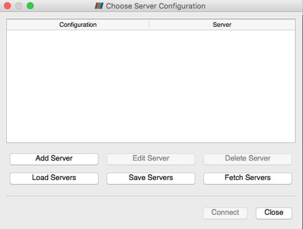
Now click the Add Server button to create a new path, which we will
construct to connect to the waiting pvserver running on your local
machine.
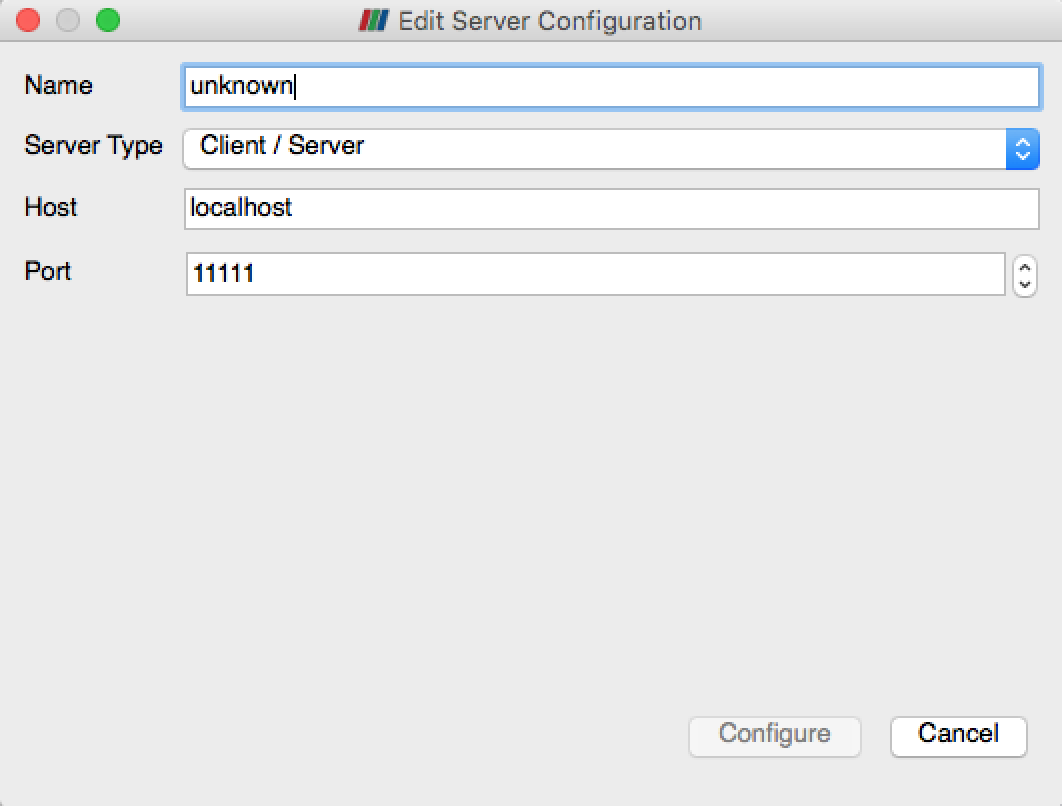
In the Edit Server Configuration Dialog, change the Name of the connection path from “unknown” to “my computer”. In actual use one would enter in a nickname for and the IP address of the remote machine we want to connect to. Now hit the Configure button.
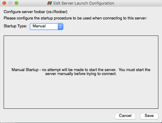
On the resulting Edit Server Launch Configuration dialog, leave the
Startup Type as Manual since we have already started a waiting
pvserver. In actual use one would typically use Command and in the
dialog enter in a script that starts up the server on the remote
machine. Click Save on the dialog to finish defining the connection.
Now that we have defined a connection, it will show up under the Choose
Server Configuration dialog whenever we hit . Click on the name of the
connection, “my computer” in this case, and click Connect to establish
the connection between the GUI and
pvserver.
Once connected, simply File → Open files on the remote system and work with them as before. To complete the exercise, open or create a dataset, and choose the vtkProcessId array to examine how it is partioned across the distributed memory of the server.
In practice, the syntax of starting up a parallel server on a remote
machine and connecting to it will be more involved. Typically the steps
include ssh’ing to a remote machine’s login node, submitting a job that
runs a script that requests some number of nodes and runs pvserver
under MPI on them with pvserver made to connect back to the waiting
client (instead of the reverse as above) over at least one ssh tunnel
hops. System administrators and other adventurous folk can find details
online here:
https://www.paraview.org/Wiki/Setting_up_a_ParaView_Server#Running_the_Server
https://www.paraview.org/Wiki/Reverse_connection_and_port_forwarding
On the local machine you may need helper utilities as well. XQuartz (for X11) on Mac and Putty (for ssh) on Windows are useful for starting up remote connections. These are required to complete the next exercise.
Once a connection is established the steps should be saved in scripts and configuration files. System administrators can publish these so that authorized users can simply download and use them. Several of these configuration files are hosted on the ParaView website where the ParaView client can download them from.
Exercise 4.3 (Fetching and using Connections)
Once again, click on to bring up the Choose Server Configuration dialog.
This time, hit the Fetch Servers button. This will bring up the Fetch
Server Configurations dialog box populated with a list of server definitions
from the webite. Choose one and click the Import Selected button to download
it into your ParaView preferences. The new connection is now available
just as the connection to “my computer” is.
To use the remote machine, once more click . This time choose the new
machine instead of “my machine” and click Connect. Doing so will bring
up a Connection Options for … dialog box that lets where you enter in
the parameters for your parallel session.
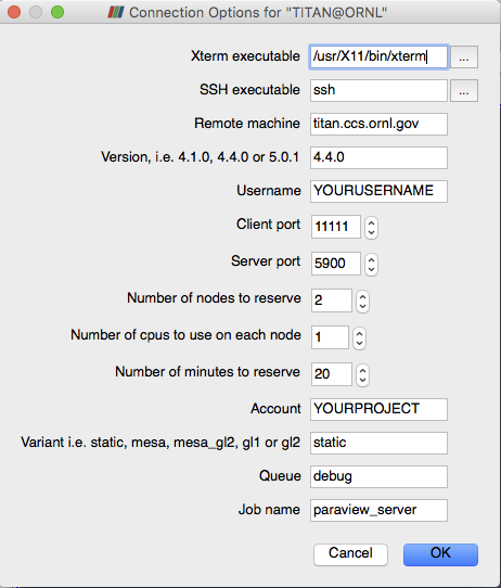
The parameters you will want to set include your username on the remote machine, the number of nodes and processes to reserve and the amount of time you want to reserve them for. Each site may have additional choices that are passed into the launch scripts on the server. Once set, click OK to try to establish a connection.
When you click OK ParaView typically spawns a terminal window (xterm on Mac and Linux, cmd.exe on Windows). Here you will have to enter in your credentials to actually access the remote machine. Once logged on, the script to reserve the nodes automatically runs and in most cases the terminal session has a menu with options for looking at the remote system’s queue. When your job reaches the top of the queue, the ParaView 3D View window will return and you can begin doing remote visualization, this time with the capacity of the remote machine at your fingertips.
4.7. Parallel Data Processing Practicalities
4.7.1. Keeping Track of Memory
When working with very large models, it is important to keep track of memory usage on the computer. One of the most common and frustrating problems encountered with large models is running out of memory. This in turn will lead to thrashing in the virtual memory system or an outright program fault.
Section 4.8.2 and Section 4.8.3 provide suggestions to reduce your memory usage. Even so, it is wise to keep an eye on the memory available in your system. ParaView provides a tool called the memory inspector designed to do just that.
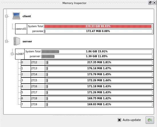
To access the memory inspector, select in the menu bar View → Memory Inspector. The memory inspector provides information for both the client you are running on and any server you might be connected to. It will tell you the total amount of memory used on the system and the amount of memory ParaView is using. For servers containing multiple nodes, information both for the conglomerate job and for each individual node are given. Note that a memory issue in any single node can cause a problem for the entire ParaView job.
4.7.2. Ghost Levels
Unfortunately, blindly running visualization algorithms on partitions of cells does not always result in the correct answer. As a simple example, consider the external faces algorithm. The external faces algorithm finds all cell faces that belong to only one cell, thereby identifying the boundaries of the mesh. What happens when we run external faces independently on our partitions?
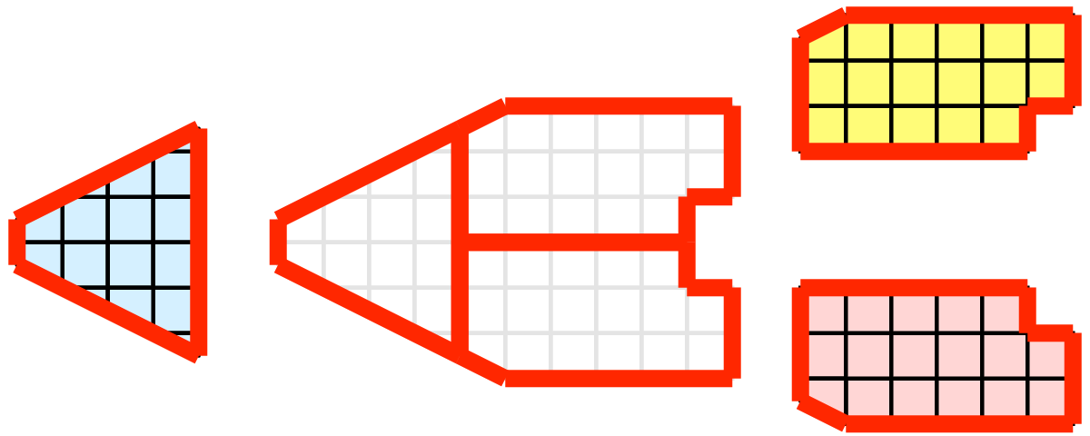
Oops. We see that when all the processes ran the external faces algorithm independently, many internal faces were incorrectly identified as being external. This happens where a cell in one partition has a neighbor in another partition. A process has no access to cells in other partitions, so there is no way of knowing that these neighboring cells exist.
The solution employed by ParaView and other parallel visualization systems is to use ghost cells (sometimes also called halo regions). Ghost cells are cells that are held in one process but actually belong to another. To use ghost cells, we first have to identify all the neighboring cells in each partition. We then copy these neighboring cells to the partition and mark them as ghost cells, as indicated with the gray colored cells in the following example.
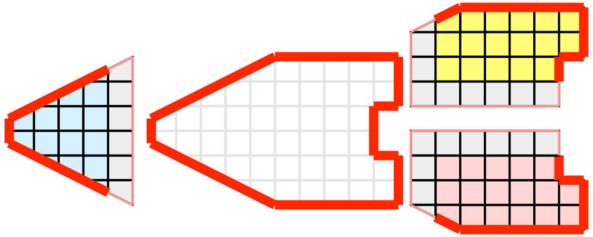
When we run the external faces algorithm with the ghost cells, we see that we are still incorrectly identifying some internal faces as external. However, all of these misclassified faces are on ghost cells, and the faces inherit the ghost status of the cell it came from. ParaView then strips off the ghost faces and we are left with the correct answer.
In this example we have shown one layer of ghost cells: only those cells that are direct neighbors of the partition’s cells. ParaView also has the ability to retrieve multiple layers of ghost cells, where each layer contains the neighbors of the previous layer not already contained in a lower ghost layer or the original data itself. This is useful when we have cascading filters that each require their own layer of ghost cells. They each request an additional layer of ghost cells from upstream, and then remove a layer from the data before sending it downstream.
4.7.3. Data Partitioning
For the most part, ParaView leaves the task of breaking up or partitioning the data to the simulation code that produced the data. It is then the responsibility of ParaView’s specific reader module for the file format in question to work efficiently, typically reading different files from different nodes independently but simultaneously. In ideal cases the rest of the parallel pipeline also operates independently and simultaneously.
Still, in the general case, since we are breaking up and distributing our data, it is prudent to address the ramifications of how we partition the data. The data shown in Section 4.1 has a spatially coherent partitioning. That is, all the cells of each partition are located in a compact region of space. There are other ways to partition data. For example, you could have a random partitioning.
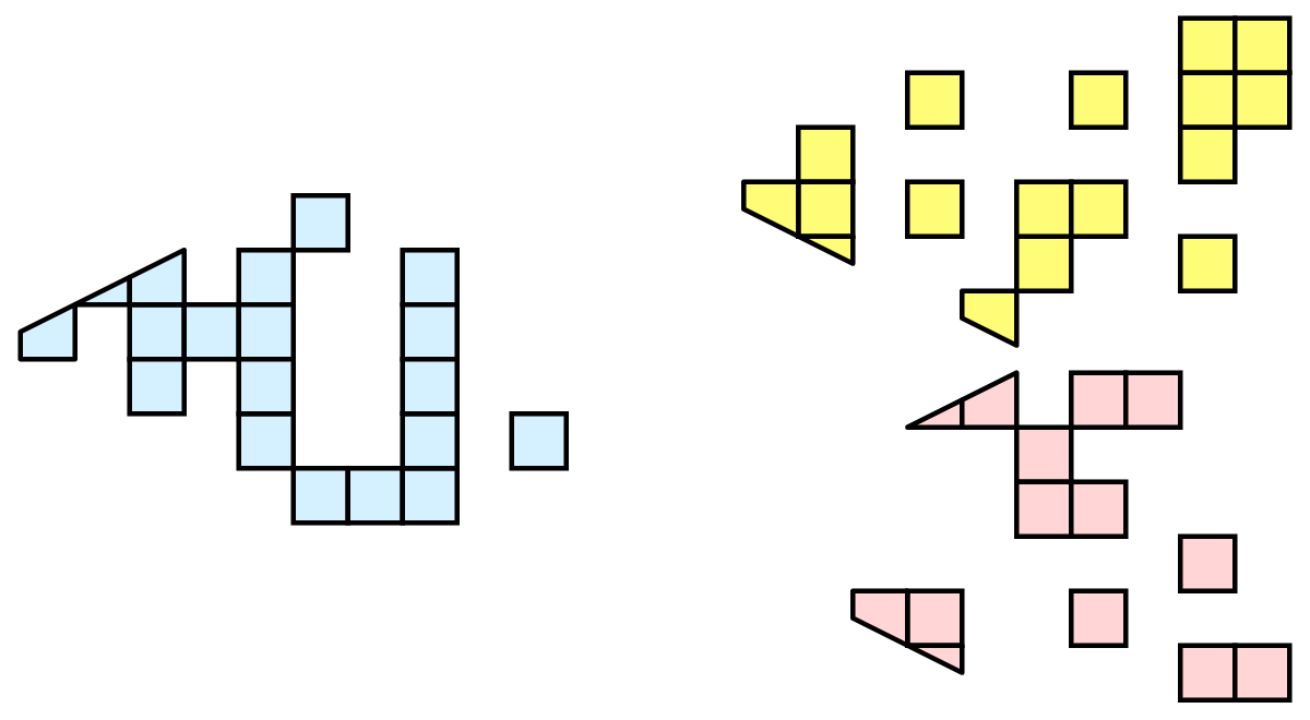
Random partitioning has some nice features. It is easy to create and is friendly to load balancing. However, a serious problem exists with respect to ghost cells.
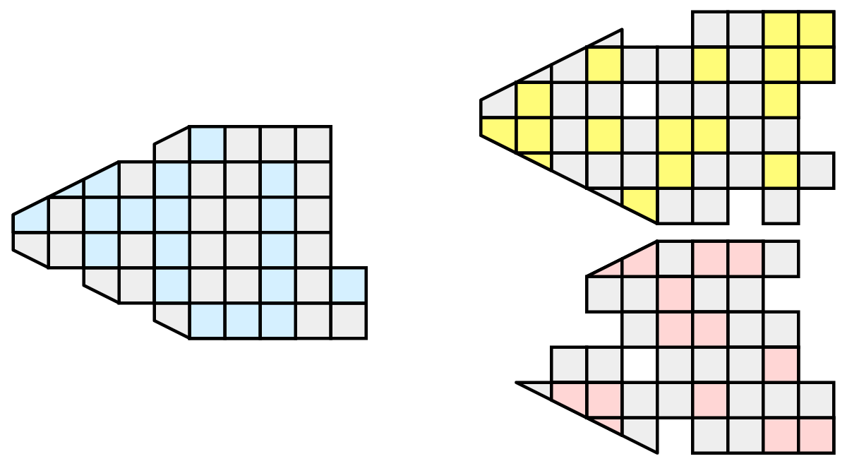
In this example, we see that a single level of ghost cells nearly replicates the entire dataset on all processes. We have thus removed any advantage we had with parallel processing. Because ghost cells are used so frequently, random partitioning is not used in ParaView.
4.7.4. D3 Filter
The previous sections described the importance of load balancing and ghost levels for parallel visualization. This section describes how to achieve that.
Load balancing and ghost cells are handled automatically by ParaView when you are reading structured data (image data, rectilinear grid, and structured grid). The implicit topology makes it easy to break the data into spatially coherent chunks and identify where neighboring cells are located.
It is an entirely different matter when you are reading in unstructured data (poly data and unstructured grid). There is no implicit topology and no neighborhood information available. ParaView is at the mercy of how the data was written to disk. Thus, when you read in unstructured data there is no guarantee about how well load balanced your data will be. It is also unlikely that the data will have ghost cells available, which means that the output of some filters may be incorrect.
Fortunately, ParaView has a filter that will both balance your unstructured data and create ghost cells. This filter is called D3, which is short for distributed data decomposition. Using D3 is easy; simply attach the filter (located in Filters → Alphabetical → D3) to whatever data you wish to repartition.
|
|
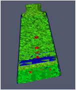
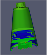
The most common use case for D3 is to attach it directly to your unstructured grid reader. Regardless of how well load balanced the incoming data might be, it is important to be able to retrieve ghost cells so that subsequent filters will generate the correct data. The example above shows a cutaway of the extract surface filter on an unstructured grid. On the left we see that there are many faces improperly extracted because we are missing ghost cells. On the right the problem is fixed by first using the D3 filter.
4.7.5. Ghost Cells Generator Filter
In many cases a better alternative to D3 filter is the Ghost Level Generator. This filter is more efficient than the D3 filter because it makes the assumption that the input unstructured grid data is already partitioned into spatially coherent regions. This is generally a safe assumption as simulations benefit from coherency too. Because of this, it concerns itself only with cells at and near the external shell of the mesh, and does not consider or transfer the bulk of the data at the interior.
4.8. Advice
4.8.1. Matching Job Size to Data Size
How many cores should I have in my |ParaView| server? This is a common question with many important ramifications. It is also an enormously difficult question. The answer depends on a wide variety of factors including what hardware each processor has, how much data is being processed, what type of data is being processed, what type of visualization operations are being done, and your own patience.
Consequently, we have no hard answer. We do however have several rules of thumb.
If you are loading structured data (image data, rectilinear grid, structured grid), try to have a minimum of one core per 20 million cells. If you can spare the cores, one core for every 5 to 10 million cells is usually plenty.
If you are loading unstructured data (poly data, unstructured grid), try to have a minimum of one core per 1 million cells. If you can spare the cores, one core for every 250 to 500 thousand cells is usually plenty.
As stated before, these are just rules of thumb, not absolutes. You should always try to experiment to gage what your core to data size should be. And, of course, there will always be times when the data you want to load will stretch the limit of the resources you have available. When this happens, you will want to make sure that you avoid data explosion and that you cull your data quickly.
4.8.2. Avoiding Data Explosion
The pipeline model that ParaView presents is very convenient for exploratory visualization. The loose coupling between components provides a very flexible framework for building unique visualizations, and the pipeline structure allows you to tweak parameters quickly and easily.
The downside of this coupling is that it can have a larger memory footprint. Each stage of this pipeline maintains its own copy of the data. Whenever possible, ParaView performs shallow copies of the data so that different stages of the pipeline point to the same block of data in memory. However, any filter that creates new data or changes the values or topology of the data must allocate new memory for the result. If ParaView is filtering a very large mesh, inappropriate use of filters can quickly deplete all available memory. Therefore, when visualizing large datasets, it is important to understand the memory requirements of filters.
Please keep in mind that the following advice is intended only for when dealing with very large amounts of data and the remaining available memory is low. When you are not in danger of running out of memory, ignore all of the following advice.
When dealing with structured data, it is absolutely important to know what filters will change the data to unstructured. Unstructured data has a much higher memory footprint, per cell, than structured data because the topology must be explicitly written out. There are many filters in ParaView that will change the topology in some way, and these filters will write out the data as an unstructured grid, because that is the only dataset that will handle any type of topology that is generated. The following list of filters will write out a new unstructured topology in its output that is roughly equivalent to the input. These filters should never be used with structured data and should be used with caution on unstructured data.
Append Datasets
Append Geometry
Clean
Clean to Grid
Connectivity
D3
Delaunay 2D/3D
Extract Edges
Linear Extrusion
Loop Subdivision
Reflect
Rotational Extrusion
Shrink
Smooth
Subdivide
Tessellate
Tetrahedralize
Triangle Strips
Triangulate
Technically, the Ribbon and Tube filters should fall into this list. However, as they only work on 1D cells in poly data, the input data is usually small and of little concern.
This similar set of filters also output unstructured grids, but they also tend to reduce some of this data. Be aware though that this data reduction is often smaller than the overhead of converting to unstructured data. Also note that the reduction is often not well balanced. It is possible (often likely) that a single process may not lose any cells. Thus, these filters should be used with caution on unstructured data and extreme caution on structured data.
Similar to the items in the preceding list, Extract Subset performs
data reduction on a structured dataset, but also outputs a structured
dataset. So the warning about creating new data still applies, but you
do not have to worry about converting to an unstructured grid.
This next set of filters also outputs unstructured data, but it also performs a reduction on the dimension of the data (for example 3D to 2D), which results in a much smaller output. Thus, these filters are usually safe to use with unstructured data and require only mild caution with structured data.
Cell Centers
Extract CTH Parts
Extract Surface
Feature Edges
Mask Points
Outline (curvilinear)
These filters do not change the connectivity of the data at all. Instead, they only add field arrays to the data. All the existing data is shallow copied. These filters are usually safe to use on all data.
Block Scalars
Cell Data to Point Data
Curvature
Elevation
Generate Surface Normals
Gradient
Level Scalars
Median
Mesh Quality
Octree Depth Limit
Octree Depth Scalars
Point Data to Cell Data
Process Id Scalars
Python Calculator
Random Vectors
Resample with dataset
Surface Flow
Surface Vectors
Texture Map to…
Transform
Warp (scalar)
This final set of filters are those that either add no data to the output (all data of consequence is shallow copied) or the data they add is generally independent of the size of the input. These are almost always safe to add under any circumstances (although they may take a lot of time).
Annotate Time
Append Attributes
Extract Block
Integrate Variables
Normal Glyphs
Outline
Outline Corners
Plot Global Variables Over Time
Temporal Shift Scale
Temporal Snap-to-Time-Steps
Temporal Statistics
There are a few special case filters that do not fit well into any of the previous classes. Some of the filters, currently Temporal Interpolator and Particle Tracer, perform calculations based on how data changes over time. Thus, these filters may need to load data for two or more instances of time, which can double or more the amount of data needed in memory. The Temporal Cache filter will also hold data for multiple instances of time. Also keep in mind that some of the temporal filters such as the temporal statistics and the filters that plot over time may need to iteratively load all data from disk. Thus, it may take an impractically long amount of time even though it does not require any extra memory.
The Programmable Filter is also a special case that is impossible to
classify. Since this filter does whatever it is programmed to do, it can
fall into any one of these categories.
4.8.3. Culling Data
When dealing with large data, it is clearly best to cull out data whenever possible, and the earlier the better. Most large data starts as 3D geometry and the desired geometry is often a surface. As surfaces usually have a much smaller memory footprint than the volumes that they are derived from, it is best to convert to a surface soon. Once you do that, you can apply other filters in relative safety.
A very common visualization operation is to extract isosurfaces from a
volume using the Contour filter. The Contour filter usually outputs
geometry much smaller than its input. Thus, the Contour filter should be
applied early if it is to be used at all. Be careful when setting up the
parameters to the Contour filter because it still is possible for it to
generate a lot of data. This obviously can happen if you specify many
isosurface values. High frequencies such as noise around an isosurface
value can also cause a large, irregular surface to form.
Another way to peer inside of a volume is to perform a Slice on it. The
Slice
filter will intersect a volume with a plane and allow you to see
the data in the volume where the plane intersects. If you know the
relative location of an interesting feature in your large dataset,
slicing is a good way to view it.
If you have little a-priori knowledge of your data and would like to
explore the data without paying the memory and processing time for the
full dataset, you can use the Extract Subset filter to subsample the
data. The subsampled data can be dramatically smaller than the original
data and should still be well load balanced. Of course, be aware that
you may miss small features if the subsampling steps over them and that
once you find a feature you should go back and visualize it with the
full dataset.
There are also several features that can pull out a subset of a volume:
Clip , Threshold
, Extract Selection
,
and Extract Subset
can all extract cells based on some criterion.
Be aware, however, that the extracted cells are almost never well balanced; expect
some processes to have no cells removed. Also, all of these filters with the exception
of Extract Subset
will convert structured data types to unstructured
grids. Therefore, they should not be used unless the extracted cells are
of at least an order of magnitude less than the source data.
When possible, replace the use of a filter that extracts 3D data with
one that will extract 2D surfaces. For example, if you are interested in
a plane through the data, use the Slice filter rather than the Clip
filter. If you are interested in knowing the location of a region of
cells containing a particular range of values, consider using the
Contour
filter to generate surfaces at the ends of the range rather
than extract all of the cells with the Threshold
filter. Be aware that
substituting filters can have an effect on downstream filters. For
example, running the Histogram
 filter after Threshold
 will
have an entirely different effect than running it after the roughly equivalent
Contour
filter.
4.8.4. Downsamplng
Downsampling is also frequently helpful for very large data. For example, the Extract Subset filter reduce the size of Structured DataSets by simpling taking strided samples along the i, j and k axes.
For unstructured grids the Quadric Clustering filter downsamples unstructured data into a smaller dataset with similar appearance by averaging vertices within cells of a grid. ParaView injects this algorithm into the display pipeline while you interact with the camera as described in the next section.
In some cases though, it can be more effective to work with structured data than unstructured data. In particular structured data volume rendering algorithms are usually much faster. In general structured data representations are very compact, adding very little overhead to the raw data values. Unstructured data types require 12 bytes of memory storage for every vertex and at least 8 bytes of storage to define each cell beyond the normal storage for cell and point aligned values. Structured types use a total of 36 bytes to represent the entire set of vertices and cells in comparison.
Fortunately you can convert from unstructured to structured easily with the Resample To Image filter. When the sizes of the cells in the input do not very widely, and can thus be approximated well by constant sized voxels, this can be very effective. This filter internally makes use of the DIY2 block-parallel communication and computation library to communicate and transfer data among the parallel nodes.
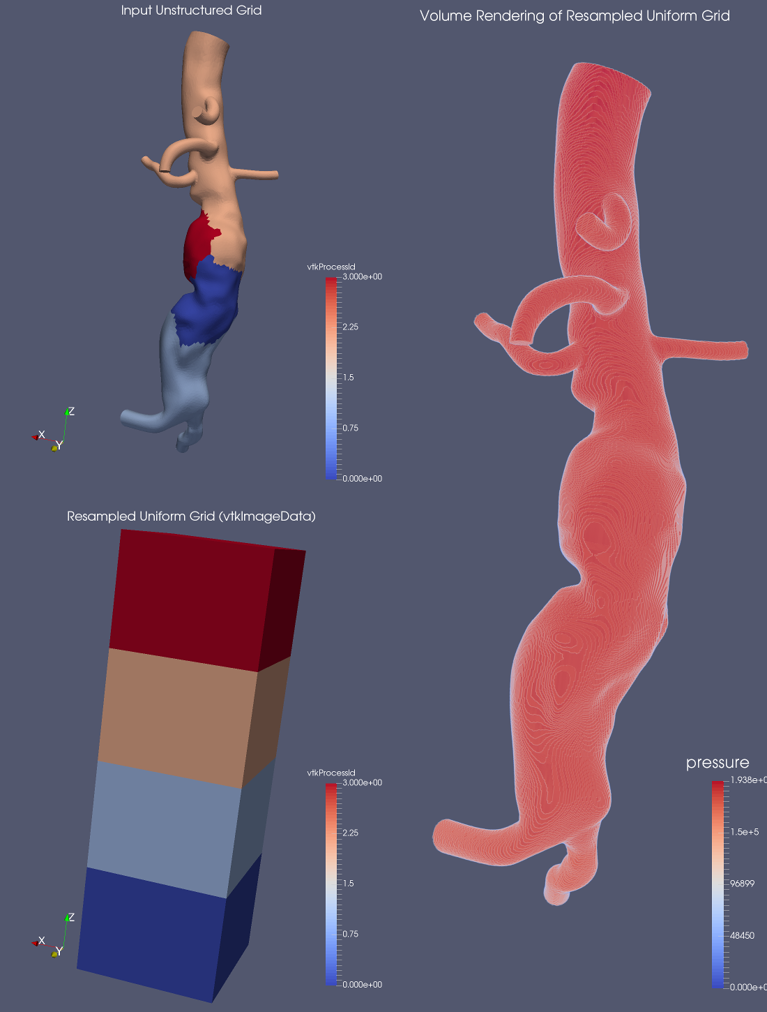
There is a companion filter Resample With DataSet which takes in a source and an input object and resamples values from the source onto the input, which does not have to be a regular grid. This also uses DIY2. This is used to assigning new values onto a particular shaped object.
4.9. Parallel Rendering Details
Rendering is the process of synthesizing the images that you see based on your data. The ability to effectively interact with your data depends highly on the speed of the rendering. Thanks to advances in 3D hardware acceleration, fueled by the computer gaming market, we have the ability to render 3D quickly even on moderately priced computers. But, of course, the speed of rendering is proportional to the amount of data being rendered. As data gets bigger, the rendering process naturally gets slower.
To ensure that your visualization session remains interactive, ParaView supports two modes of rendering that are automatically flipped as necessary. In the first mode, still render, the data is rendered at the highest level of detail. This rendering mode ensures that all of the data is represented accurately. In the second mode, interactive render, speed takes precedence over accuracy. This rendering mode endeavors to provide a quick rendering rate regardless of data size.
While you are interacting with a 3D view, for example rotating, panning, or zooming with the mouse, ParaView uses an interactive render. This is because during the interaction a high frame rate is necessary to make these features usable and because each frame is immediately replaced with a new rendering while the interaction is occurring so that fine details are less important during this mode. At any time when interaction of the 3D view is not taking place, ParaView uses a still render so that the full detail of the data is available as you study it. As you drag your mouse in a 3D view to move the data, you may see an approximate rendering while you are moving the mouse, but the full detail will be presented as soon as you release the mouse button.
The interactive render is a compromise between speed and accuracy. As such, many of the rendering parameters concern when and how lower levels of detail are used.
4.9.1. Basic Rendering Settings
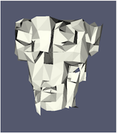
Some of the most important rendering options are the LOD parameters. During interactive rendering, the geometry may be replaced with a lower level of detail (LOD), an approximate geometry with fewer polygons.
|
|
|
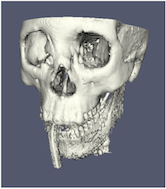
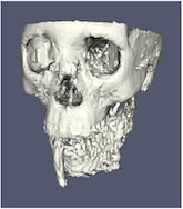
The resolution of the geometric approximation can be controlled. In the proceeding images, the left image is the full resolution; the middle image is the default decimation for interactive rendering, and the right image is ParaView’s maximum decimation setting.
The 3D rendering parameters are located in the settings dialog box which is accessed in the menu from Edit → Settings (ParaView → Preferences on the Mac). The rendering options in the dialog are in the Render View tab.
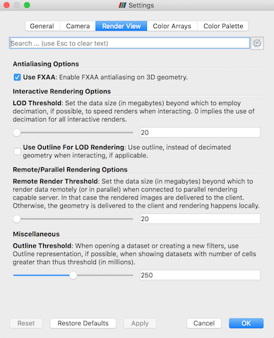
The options pertaining to the geometric decimation for interactive
rendering are located in a section labeled Interactive Rendering
Options. Some of these options are considered advanced, so to access
them you have to either toggle on the advanced options with the
button or search for the option using the edit box at the top of the dialog.
The interactive rendering options include the following.
Set the data size at which to use a decimated geometry in interactive rendering. If the geometry size is under this threshold, ParaView always renders the full geometry. Increase this value if you have a decent graphics card that can handle larger data. Try decreasing this value if your interactive renders are too slow.
Set the factor that controls how large the decimated geometry should be. This control is set to a value between 0 and 1. 0 produces a very small number of triangles but possibly with a lot of distortion. 1 produces more detailed surfaces but with larger geometry.
Add a delay between an interactive render and a still render. ParaView usually performs a still render immediately after an interactive motion is finished (for example, releasing the mouse button after a rotation). This option can add a delay that can give you time to start a second interaction before the still render starts, which is helpful if the still render takes a long time to complete.
Use an outline in place of decimated geometry. The outline is an alternative for when the geometry decimation takes too long or still produces too much geometry. However, it is more difficult to interact with just an outline.
ParaView contains many more rendering settings. Here is a summary of some other settings that can effect the rendering performance regardless of whether ParaView is run in client-server mode or not. These options are spread among several categories, and several are considered advanced.
Geometry Mapper Options
Enable or disable the use of display lists. Display lists are internal structures built by graphics systems. They can potentially speed up rendering but can also take up memory.
Translucent Rendering Options
Enable or disable depth peeling. Depth peeling is a technique ParaView uses to properly render translucent surfaces. With it, the top surface is rendered and then “peeled away” so that the next lower surface can be rendered and so on. If you find that making surfaces transparent really slows things down or renders completely incorrectly, then your graphics hardware may not be implementing the depth peeling extensions well; try shutting off depth peeling.
Set the maximum number of peels to use with depth peeling. Using more peels allows more depth complexity but allowing less peels runs faster. You can try adjusting this parameter if translucent geometry renders too slow or translucent images do not look correct.
Miscellaneous
When creating very large datasets, default to the outline representation. Surface representations usually require ParaView to extract geometry of the surface, which takes time and memory. For data with size above this threshold, use the outline representation, which has very little overhead, by default instead.
Show or hide annotation providing rendering performance information. This information is handy when diagnosing performance problems.
Note that this is not a complete list of ParaView rendering settings. We have left out settings that do not significantly effect rendering performance. We have also left out settings that are only valid for parallel client-server rendering, which are discussed in Section 4.9.3.
4.9.2. Image Level of Detail
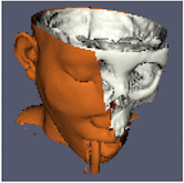
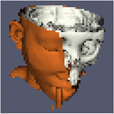
The overhead incurred by the parallel rendering algorithms is proportional to the size of the images being generated. Also, images generated on a server must be transfered to the client, a cost that is also proportional to the image size. To help increase the frame rate during interaction, ParaView introduces a new LOD parameter that controls the size of the images.
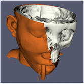
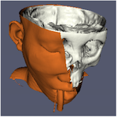
During interaction while parallel rendering, ParaView can optionally subsample the image. That is, ParaView will reduce the resolution of the image in each dimension by a factor during interaction. Reduced images will be rendered, composited, and transfered. On the client, the image is inflated to the size of the available space in the GUI.
|
|
|
|
The resolution of the reduced images is controlled by the factor with which the dimensions are divided. In the preceding images, the left image has the full resolution. The following images were rendered with the resolution reduced by a factor of 2, 4, and 8, respectively.
ParaView also has the ability to compress images before transferring them from server to client. Compression, of course, reduces the amount of data transferred and therefore makes the most of the available bandwidth. However, the time it takes to compress and decompress the images adds to the latency.
ParaView contains three different image compression algorithms for client-server rendering. The oldest is a custom algorithm called Squirt, which stands for Sequential Unified Image Run Transfer. Squirt is a run-length encoding compression that reduces color depth to increase run lengths. The second algorithm uses the Zlib compression library, which implements a variation of the Lempel-Ziv algorithm. Zlib typically provides better compression than Squirt, but takes longer to perform and hence adds to the latency. The most recent addition is the LZ4 algorithm which is tuned for fast compression and decompression.
4.9.3. Parallel Render Parameters
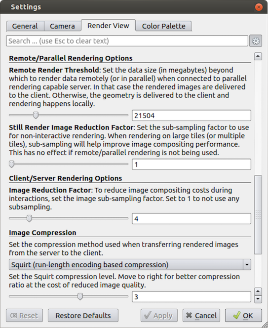
Like the other 3D rendering parameters, the parallel rendering parameters are located in the settings dialog box, which is accessed in the menu from Edit → Settings (ParaView → Preferences on the Mac). The parallel rendering options in the dialog are in the Render View tab (intermixed with several other rendering options such as those described in Section 4.9.1). The parallel and client-server options are divided among several categories, and several are considered advanced.
Remote/Parallel Rendering Options
Set the data size at which to render remotely in parallel or to render locally. If the geometry is over this threshold (and ParaView is connected to a remote server), the data is rendered in parallel remotely and images are sent back to the client. If the geometry is under this threshold, the geometry is sent back to the client and images are rendered locally on the client.
Set the sub-sampling factor for still (non-interactive) rendering. Some large displays have more resolution than is really necessary, so this sub-sampling reduces the resolution of all images displayed.
Client/Server Rendering Options
Set the interactive subsampling factor. The overhead of parallel rendering is proportional to the size of the images generated. Thus, you can speed up interactive rendering by specifying an image subsampling rate. When this box is checked, interactive renders will create smaller images, which are then magnified when displayed. This parameter is only used during interactive renders.
Image Compression
Before images are shipped from server to client, they optionally can be compressed using one of the three compression algorithms: Squirt, Zlib or LZ4. To make the compression more effective, each algorithm has one or more tunable parameters that let you customize the behavior and target level of compression.
Suggested image compression presets are provided for several common network types. When attempting to select the best image compression options, try starting with the presets that best match your connection.
4.9.4. Parameters for Large Data
The default rendering parameters are suitable for most users. However, when dealing with very large data, it can help to tweak the rendering parameters. The optimal parameters depend on your data and the hardware ParaView is running on, but here are several pieces of advice that you should follow.
Try turning off display lists. Turning this option off will prevent the graphics system from building special rendering structures. If you have graphics hardware, these rendering structures are important for feeding the GPUs fast enough. However, if you do not have GPUs, these rendering structures do not help much.
If there is a long pause before the first interactive render of a particular dataset, it might be the creation of the decimated geometry. Try using an outline instead of decimated geometry for interaction. You could also try lowering the factor of the decimation to 0 to create smaller geometry.
Avoid shipping large geometry back to the client. The remote rendering will use the power of entire server to render and ship images to the client. If remote rendering is off, geometry is shipped back to the client. When you have large data, it is always faster to ship images than to ship data (although if your network has a high latency, this could become problematic for interactive frame rates).
Adjust the interactive image sub-sampling for client-server rendering as needed. If image compositing is slow, if the connection between client and server has low bandwidth, or if you are rendering very large images, then a higher subsample rate can greatly improve your interactive rendering performance.
Make sure Image Compression is on. It has a tremendous effect on desktop delivery performance, and the artifacts it introduces, which are only there during interactive rendering, are minimal. Lower bandwidth connections can try using Zlib or LZ4 instead of Squirt compression. Zlib will create smaller images at the cost of longer compression/decompression times.
If the network connection has a high latency, adjust the parameters to avoid remote rendering during interaction. In this case, you can try turning up the remote rendering threshold a bit, and this is a place where using the outline for interactive rendering is effective.
If the still (non-interactive) render is slow, try turning on the delay between interactive and still rendering to avoid unnecessary renders.
4.10. Catalyst
For small scale data, running the ParaView GUI in serial mode is likely acceptable. For large scale data, interactive parallel visualization is quite useful. For very large scale data, batch mode parallel processing is more effective because of practical concerns like batch system queue wait time before a parallel job is launched and system policies that limit the size and duration of interactive jobs.
For extreme scale visualization even batch mode is beginning to be impractical though as comparatively slow disks limit the size of data that can be saved off by the simulation at runtime. In this domain ParaView’s Catalyst configuration is recommended as an in situ analysis and visualization library.
Catalyst is a visualization framework that packages either portions or the entirety of ParaView’s parallel server framework so that it can be linked into and called from arbitrary simulation codes. Slow IO systems are largely bypassed via an adaptor mechanism whereby the simulation code’s data structures are translated or ideally reused directly by ParaView while still in RAM.
With Catalyst, full resolution simulation products stay in memory instead of being saved to and later loaded back from disk. As the simulation progresses, it periodically calls into ParaView. In this way it is possible to immediately generate smaller derived datasets, images, plots, etc. that would otherwise be generated during post processing after a much longer, human in the loop, delay.

As explained more fully in the ParaView Catalyst User’s Guide there are two components to making use of Catalyst. The first is to Catalyze the simulation. This is where a software developer compiles Catalyst into the simulation, adds a handful of (typically three) function calls to it, and fleshes out an adaptor template with working code that produces VTK datasets from the simulation’s own internal data structures.
Once the simulation has been Catalyzed, day to day users need to define what ParaView should do with the data it is given. Catalyst can produce data extracts, images, statistical quantities, etc. Any of these can be made with Python or even lower level Fortran, C or C++ coding to maximize runtime efficiency, but it is more flexible and convenient to do so with recorded Catalyst scripts which are demonstrated in the next exercise.
With Catalyst scripts the simulation input deck references a Python file that defines the visualization pipeline. The script can do nearly everything that ParaView batch scripts do and is generally created with help from the ParaView GUI. To create the script one loads a representative dataset, creates a pipeline, designates the set of inputs and outputs to and output from the pipeline, and then simply saves out the Python file. Catalyst scripts are very similar to recorded Python traces.
The user interface for defining the inputs and outputs is found inside the the Catalyst Script Generator plugin. Our final exercise demonstrates with a small example.
Exercise 4.4 (Catalyst)
We demonstrate a Catalyst workflow using the ParaView binaries and the PythonFullExample code from the ParaView source tree. PythonFullExample is a toy simulation that uses numpy and mpi4py to update a regular grid as time evolves. The example consists of four files. Open and read these to begin.
The computational kernel is in fedatastructures.py. Inspection of the code shows that it has no particular dependency on ParaView, and simply makes up a structured grid in parallel with numpy and mpi4py.
From fedatastructures.py:
def Update(self, time):
   self.Velocity =
   numpy.zeros((self.Grid.GetNumberOfPoints(), 3))
   self.Velocity = self.Velocity + time
   self.Pressure = numpy.zeros(self.Grid.GetNumberOfCells())
The main loop is found in the fedriver.py. If the doCoprocessing variable is false, this falls back to a simple loop which runs the simulation to update the in-memory array over time. When the variable is true the Catalyst library is exercised via three function calls: initialize(), coprocess() and finalize().
From fedriver.py:
import numpy
import sys
from mpi4py import MPI

comm = MPI.COMM_WORLD
rank = comm.Get_rank()

import fedatastructures

grid = fedatastructures.GridClass([10, 12, 10], [2, 2, 2])
attributes = fedatastructures.AttributesClass(grid)
doCoprocessing = True

if doCoprocessing:
    import coprocessor
    coprocessor.initialize()
    coprocessor.addscript("cpscript.py")

for i in range(100):
    attributes.Update(i)
    if doCoprocessing:
        import coprocessor
        coprocessor.coprocess(i, i, grid, attributes)

if doCoprocessing:
    import coprocessor
    coprocessor.finalize()
fedriver.py and fedatastructures.py represent the simulation code. The Catalyst parts consist of the general purpose adaptor code, found within the coprocessor.py, and the pipeline definition, found in cpscript.py. In coprocessor.py note in particular where the coprocess function populates the dataDescription data structure to give fedatastructure’s content over to ParaView. The coprocessor also takes in, with the addscript() call, the pipeline definition file.
From coprocessing.py:
if coProcessor.RequestDataDescription(dataDescription):
    import fedatastructures
    imageData = vtk.vtkImageData()
    imageData.SetExtent(\
      grid.XStartPoint, grid.XEndPoint, \
      0, grid.NumberOfYPoints-1, \
      0, grid.NumberOfZPoints-1)
    imageData.SetSpacing(grid.Spacing)

    velocity = paraview.numpy_support.numpy_to_vtk(attributes.Velocity)
    velocity.SetName("velocity")
    imageData.GetPointData().AddArray(velocity)

    pressure = numpy_support.numpy_to_vtk(attributes.Pressure)
    pressure.SetName("pressure")
    imageData.GetCellData().AddArray(pressure)
The starting script for this example is called cpscript.py. This simply saves out the input it is given in a format that the ParaView GUI can readily understand. The internals of the PipelineClass is essentially a ParaView batch script that takes as input not a file but the datadescription class from the adaptor.
From cpscript.py:
class Pipeline:
   filename_6_pvti = \
       coprocessor.CreateProducer( datadescription, "input" )

   # create a new 'Parallel ImageData Writer'
   imageDataWriter1 = \
       servermanager.writers.XMLPImageDataWriter(Input=filename_6_pvti)

   # register the writer with coprocessor
   # and provide it with information such as the filename to use,
   # how frequently to write the data, etc.
   coprocessor.RegisterWriter(imageDataWriter1, \
       filename="fullgrid_%t.pvti", freq=100)

   Slice1 = Slice( \
       Input=filename_6_pvti, guiName="Slice1", \
       Crinkleslice=0, SliceOffsetValues=[0.0], \
       Triangulatetheslice=1, SliceType="Plane" )
   Slice1.SliceType.Offset = 0.0
   Slice1.SliceType.Origin = [9.0, 11.0, 9.0]
   Slice1.SliceType.Normal = [1.0, 0.0, 0.0]

   # create a new 'Parallel PolyData Writer'
   parallelPolyDataWriter1 = \
       servermanager.writers.XMLPPolyDataWriter(Input=Slice1)

   # register the writer with coprocessor
   # and provide it with information such as the filename to use,
   # how frequently to write the data, etc.
   coprocessor.RegisterWriter(\
       parallelPolyDataWriter1, filename='slice_%t.pvtp', freq=10)

   return Pipeline()
Now let us run the simulation code to produce some data.
On Mac:
/Applications/ParaView-x.x.x.app/Contents/MacOS/mpiexec -np 2 /Applications/ParaView-x.x.x.app/Contents/bin/pvbatch –symmetric fedriver.pyOn Linux:
/usr/local/lib/paraview-x.x.x/mpiexec -np 2 /usr/local/bin/pvbatch –symmetric fedriver.pyOn Windows:
mpiexec -np 2 "C:/Program Files/ParaView x.x.x/bin/pvbatch" –symmetric fedriver.py
The example will run and produce several files, among them fullgrid_0.pvti which is a raw dump of the simulation’s full output. Let us use that to customize Catalyst’s output.
First open the file in the ParaView GUI and inspect it. You will find that this is a very simple structured grid with two variables, pressure and velocity. Now insert the File → Extract Subset filter into the pipeline to demonstrate some simple but useful processing.
Next let’s use the Export Inspector to declare a set of files that you want Catalyst to produce at run time. As we will see in a moment, the ParaView GUI is able to generate Catalyst scripts by capturing the current state of the visualization constructed in ParaView. However, the state does not include file creation, which is typically done in interactive sessions via File → Save Data or File → Save Screenshot actions.
Since ParaView 5.6, the Export Inspector is the place for defining Catalyst’s data products. Open it by clicking Export Inspector under the Catalyst menu. By default the panel will show up in a new tab near the Properties Panel. Select it, if necessary, to bring it to the front.
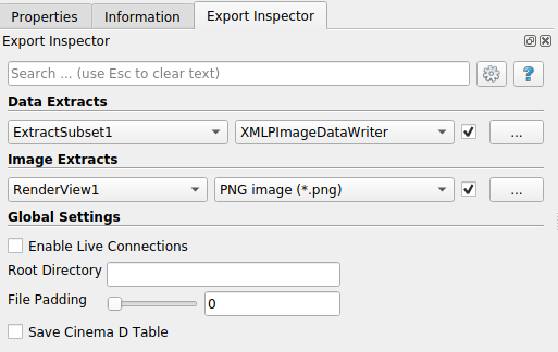
The Data Extracts section at the top allows you to attach a writer to the currently active element within the visualization pipeline. Make sure ExtractSubset1 is selected in the Pipeline Browser and then choose XMLPImageDataWriter from the file format pull down to the right of this filter name in Data Extracts. To confirm that you want Catalyst to perform this particular data export at run time, click on the checkbox to the right of the file format.
If you want to change the writer’s default settings, click on the configure button with the … label to the right of the checkbox. In the Save Data Options dialog that pops up, you can control things like the compression level, the frequency at which Catalyst generates files, and the filename. The default filename is composed from the producing filter’s name, the time step and the file format extension. Let’s change it from “ExtractSubset1_%t.pvti” to “smallgrid_%t.pvti”. Here “%t” gets replaced with the iteration number when the simulation runs. Later, when we run the simulation with this script, we will get subsampled results instead of the full grid.
To add rendered images to the simulation run, configure them with the Image Extracts section of the Export Inspector. Just like with data extracts, you configure outputs for the currently active view here. Do so by making sure that “RenderView1” is active and then hit the checkbox to enable png dumps of this view.
To save your visualization session in the form of a Catalyst script, click Catalyst → Export Catalyst Script. Note that all of your choices in the Export Inspector are kept with the rest of the ParaView state, so File → Save State can make it easy to modify your setup after the fact.
Finally quit ParaView and run the simulation again. The files produced will now include png files for screen captures at each time step, and vti files corresponding to the output of the Extract Subset filter at each timestep. Simply repeat the process, adding filters and views for example, to set up any type of data generator for the simulation.
Note this is but one interface to using Catalyst. If simulation users are uncomfortable with ParaView and/or Python, it is entirely possible for simulation developers to instrument the simulation code with predefined and parameterized pipelines with or without resorting to Python. It is also possible to create minimized Catalyst editions that consist of just a small portion of the larger ParaView code base.
As is the case with ParaView itself, Catalyst is evolving rapidly. It already has more advanced offshoots than described here. One, is a live data capability in which one can connect a ParaView client to a running Catalyzed simulation in order to check in on its progress from time to time and do a limited amount of computational steering and debugging. Another is Cinema, which is an image based framework for deferred visualization of automatically generated simulation results organized in a database. For information on these we refer the reader to the ParaView mailing list and websites.