3. Batch Python Scripting

Python scripting can be leveraged in two ways within ParaView. First, Python scripts can automate the setup and execution of visualizations by performing the same actions as a user at the GUI. Second, Python scripts can be run inside pipeline objects, thereby performing parallel visualization algorithms. This chapter describes the first mode, batch scripting for automating the visualization.

Batch scripting is a good way to automate mundane or repetitive tasks, but it is also a critical component when using ParaView in situations where the GUI is undesired or unavailable. The automation of Python scripts allows you to leverage ParaView as a scalable parallel post-processing framework. We are also leveraging Python scripting to establish in situ computation within simulation code. (ParaView supports an in situ library called Catalyst, which is documented in Section 4.10 of this tutorial and more fully online at https://www.paraview.org/in-situ/).

This tutorial gives only a brief introduction to Python scripting. More comprehensive documentation on scripting is given in the ParaView User’s Guide. There are also further links on ParaView’s documentation web page (https://www.paraview.org/documentation) including a complete reference to the ParaView Python API.

3.1. Starting the Python Interpreter

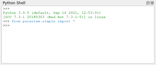
There are many ways to invoke the Python interpreter. The method you use depends on how you are using the scripting. The easiest way to get a python interpreter, and the method we use in this tutorial, is to select View → Python Shell from the menu. This will bring up a dialog box containing controls for ParaView’s Python shell. This is the Python interpreter, where you directly control ParaView via the commands described later. For convenience in typing, ParaView’s Python shell supports tab completion and history browsing with the up and down keys.

If you are most interested in getting started on writing scripts, feel free to skip to the next section past the discussion of the other ways to invoke scripting.

ParaView comes with two command line programs that execute Python scripts: pvpython and pvbatch. They are similar to the python executable that comes with Python distributions in that they accept Python scripts either from the command line or from a file and they feed the scripts to the Python interpreter.

The difference between pvpython and pvbatch is subtle and has to do with the way they establish the visualization service. pvpython is roughly equivalent to the paraview client GUI with the GUI replaced with the Python interpreter. It is a serial application that connects to a ParaView server (which can be either builtin or remote). pvbatch is roughly equivalent to pvserver except that commands are taken from a Python script rather than from a socket connection to a ParaView client. It is a parallel application that can be launched with mpirun (assuming it was compiled with MPI), but it cannot connect to another server; it is its own server. In general, you should use pvpython if you will be using the interpreter interactively and pvbatch if you are running in parallel.

It is also possible to use the ParaView Python modules from programs outside of ParaView. This can be done by pointing the PYTHONPATH environment variable to the location of the ParaView libraries and Python modules and pointing the LD_LIBRARY_PATH (on Unix/Linux), DYLD_LIBRARY_PATH (on Mac), or PATH (on Windows) environment variable to the ParaView libraries. Running the Python script this way allows you to take advantage of third-party applications such as Python’s Integrated Development and Learning Environment (IDLE). For more information on setting up your environment, consult the ParaView Wiki.

3.2. Tracing ParaView State

Before diving into the depths of the Python scripting features, let us take a moment to explore the automated facilities for creating Python scripts. The ParaView GUI’s Python Trace feature allows one to very easily create Python scripts for many common tasks. To use Trace, one simply begins a trace recording via Start Trace, found in the Tools menu, and ends a trace recording via Stop Trace, also found in the Tools menu. This produces a Python script that reconstructs the actions taken in the GUI. That script contains the same set of operations that we are about to describe. As such, Trace recordings are a good resource when you are trying to figure out how to do some action via the Python interface, and conversely the following descriptions will help in understanding the contents of any given Trace script.

Exercise 3.1 (Creating a Python Script Trace)

If you have been following an exercise in a previous section, now is a good time to reset ParaView. The easiest way to do this is to select Edit → Reset Session from the menu or hit on the toolbar.

Click the Start Trace option in the Tools menu.
A dialog box with options for the trace is presented. We will discuss the meaning of these options later. For now, just click OK.
Build a simple pipeline in the main ParaView GUI. For example, create a sphere source and then clip it.
Click Stop Trace in the Tools menu.
An editing window will open populated with a Python script that replicates the operations you just made.

Even if you have not been exposed to ParaView’s Python bindings, the commands being performed in the traced script should be familiar. Once saved to your hard drive, you can of course edit the script with your favorite editor. The final script can be interpreted by the pvpython or pvbatch program for totally automated visualization. It is also possible to run this script in the GUI. The Python Shell dialog has a Run Script button that invokes a saved script.

It should be noted that there is also a way to capture the current ParaView state as a Python script without tracing actions. Simply select Save State… from the ParaView File menu and choose to save as a Python .py state file (as opposed to a ParaView .pvsm state file). We will not have an exercise on state Python scripts, but suffice it to say they can be used in much the same way as traced Python scripts. You are welcome to experiment with this feature as you like.

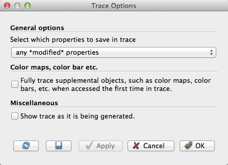
As noted earlier in the exercise, Python tracing has some options that are presented in a dialog box before the tracing starts. The first option selections what properties are saved to the trace. Some properties you explicitly set through the GUI, such as a value entered in a GUI widget. Some properties are set internally by the ParaView application, such as the initial position of a clip plane based on the bounds of the object it is being applied to. Many other properties are left at some default value. You can choose one of the following classes of properties to save:

all properties: Traces the values of all properties even if they remain at the default. This can be helpful to introspect all possible properties or to ensure a consistent state regardless of the settings for other users. This also yields a very verbose output that can be hard to read.
any *modified* properties: Ignores any properties that do not change from their defaults. This is a good option for most use cases.
only *user-modified* properties: Ignores any properties that are not explicitly set by the user. Traces of this nature rely on any internally set properties being reapplied when the script is run.

The next option has to do with supplemental objects that are managed by the ParaView GUI (or client) rather than in the server’s state. Check this box to capture all of the state associated with these objects, which includes color maps, color bars, and other annotation.

Finally, ParaView provides the option to show the trace file as it is being generated. This can be a helpful option to use when learning what Python commands can be used to replicate particular actions in the ParaView GUI.

3.3. Macros

A simple but powerful way to customize the behavior of ParaView is to add your Python script as a macro. A macro is simply an automated script that can be invoked through its button in a toolbar or its entry in the menu bar. Any Python script can be assigned to a macro.

Exercise 3.2 (Adding a Macro)

This exercise is a continuation of Exercise 3.1. You will need to finish that exercise before beginning this one. You should have the editing window containing the Python script created in Exercise 3.1 open.

In the menu bar (of the editing window), select File → Save As Macro….
Choose a descriptive name for the macro file and save it in the default directory provided by the browser. You should now see your macro on the Macro toolbar at the top of the ParaView GUI.

At this point, you should now see your macro added to the toolbars. By default, macro toolbar buttons are placed in the middle row all the way to the right. If you are short on space in your GUI, you may need to move toolbars around to see it. You will also see that your macro has been added to the Macros menu.

Close the Python editor window.
Delete the pipeline you have created by either selecting Edit → Delete All from the menu or selecting from the toolbar.
Activate your macro by clicking on the toolbar button or selecting it in the Macros menu.

In this example our macro created something from scratch. This is helpful if you often load some data in the same way every time. You can also trace the creation of filters that are applied to existing data. A macro from a trace of this nature allows you to automate the same visualization on different data.

3.4. Creating a Pipeline

As described in the previous two sections, the ParaView GUI’s Python Trace feature provides a simple mechanism to create scripts. In this section we will begin to describe the basic bindings for ParaView scripting. This is important information in building Python scripts, but you can always fall back on producing traces with the GUI.

The first thing any ParaView Python script must do is load the paraview.simple module. This is done by invoking

from paraview.simple import *

In general, this command needs to be invoked at the beginning of any ParaView batch Python script. This command is automatically invoked for you when you bring up the scripting dialog in ParaView, but you must add it yourself when using the Python interpreter in other programs (including pvpython and pvbatch).

The paraview.simple module defines a function for every source, reader, filter, and writer defined in ParaView. The function will be the same name as shown in the GUI menus with spaces and special characters removed. For example, the Sphere function corresponds to Sources → Sphere in the GUI and the PlotOverLine function corresponds to Filters → Data Analysis → Plot Over Line. Each function creates a pipeline object, which will show up in the pipeline browser (with the exception of writers), and returns an object that is a proxy that can be used to query and manipulate the properties of that pipeline object.

There are also several other functions in the paraview.simple module that perform other manipulations. For example, the pair of functions Show and Hide turn on and off, respectively, the visibility of a pipeline object in a view. The Render function causes a view to be redrawn.

To obtain a concise list of the functions available in paraview.simple, invoke dir(paraview.simple). Alternatively, as explained in Section 3.6 you can get a verbose listing via help(paraview.simple).

Exercise 3.3 (Creating and Showing a Source)

If you have been following an exercise in a previous section, now is a good time to reset ParaView. The easiest way to do this is to select from the toolbar.

If you have not already done so, open the Python shell in the ParaView GUI by selecting View → Python Shell from the menu. You will notice that the following has been added for you already.

from paraview.simple import *

Create and show a Sphere source by typing the following in the Python shell.

sphere = Sphere()
Show()
Render()
ResetCamera()

The Sphere command creates a sphere pipeline object. Once it is executed you will see an item in the pipeline browser created. We save a proxy to the pipeline object in the variable sphere. We are not using this variable (yet), but it is good practice to save references to your pipeline objects.

The subsequent Show command turns on visibility of this object in the view, and the subsequent Render causes the results to be seen. Finally, although the ParaView GUI automatically adjusts the camera to data shown for the first time, the Python scripting does not. The call to ResetCamera performs this automatic camera adjustment if necessary.

At this point you can interact directly with the GUI again. Try changing the camera angle in the view with the mouse.

Exercise 3.4 (Creating and Showing a Filter)

Creating filters is almost identical to creating sources. By default, the last created pipeline object will be set as the input to the newly created filter, much like when creating filters in the GUI.

This exercise is a continuation of Exercise 3.3. You will need to finish that exercise before beginning this one.

Type in the following script in the Python shell that hides the sphere and then adds the shrink filter to the sphere and shows that.

Hide()
shrink = Shrink()
Show()
Render()

The sphere should be replaced with the output of the Shrink filter, which makes all of the polygons smaller to give the mesh an exploded type of appearance.

So far as we have built pipelines, we have accepted the default parameters for the pipeline objects. As we have seen in the exercises of Section 2, it is common to have to modify the parameters of the objects using the properties panel.

In Python scripting, we use the proxy returned from the creation functions to manipulate the pipeline objects. These proxies are in fact Python objects with class attributes that correspond to the same properties you set in the properties panel. They have the same names as those in the properties panel with spaces and other illegal characters removed. Use dir(variable) or help(variable) to get a list of all attributes on any variable that you have access to. In most cases, simply assign values to an object’s attributes in order to change them.

Exercise 3.5 (Changing Pipeline Object Properties)

This exercise is a continuation of Exercise 3.3 and Exercise 3.4. You will need to finish those exercises before beginning this one.

Recall that we have so far created two Python variables, sphere and shrink, that are proxies to the corresponding pipeline objects. First, enter the following command into the Python shell to get a concise listing of all attributes of the sphere.

dir(sphere)

Next, enter the following command into the Python shell to get the current value of the Theta Resolution property of the sphere.

print(sphere.ThetaResolution)

The Python interpreter should respond with the result 8. (Note that using the print function, which instructs Python to output the arguments to standard out, is superfluous here as the Python shell will output the result of any command anyway.) Let us double the number of polygons around the equator of the sphere by changing this property.

sphere.ThetaResolution = 16
Render()

The shrink filter has only one property, Shrink Factor. We can adjust this factor to make the size of the polygons larger or smaller. Let us change the factor to make the polygons smaller.

shrink.ShrinkFactor = 0.25
Render()

You may have noticed that as you type in Python commands to change the pipeline object properties, the GUI in the properties panel updates accordingly.

So far we have created only non-branching pipelines. This is a simple and common case and, like many other things in the paraview.simple module, is designed to minimize the amount of work for the simple and common case but also provide a clear path to the more complicated cases. As we have built the non-branching pipeline, ParaView has automatically connected the filter input to the previously created object so that the script reads like the sequence of operations it is. However, if the pipeline has branching, we need to be more specific about the filter inputs.

Exercise 3.6 (Branching Pipelines)

This exercise is a continuation of Exercise 3.3 through Exercise 3.5. You will need to finish Exercise 3.3 and Exercise 3.4 before beginning this one (Exercise 3.5 is optional).

Recall that we have so far created two Python variables, sphere and shrink, that are proxies to the corresponding pipeline objects. We will now add a second filter to the sphere source that will extract the wireframe from it. Enter the following in the Python shell.

wireframe = ExtractEdges(Input=sphere)
Show()
Render()

An Extract Edges filter is added to the sphere source. You should now see both the wireframe of the original sphere and the shrunken polygons.

Notice that we explicitly set the input for the Extract Edges filter by providing Input=sphere as an argument to the ExtractEdges function. What we are really doing is setting the Input property upon construction of the object. Although it would be possible to create the object with the default input, and then set the input later, it is not recommended. The problem is that not all filters accept all input. If you initially create a filter with the wrong input, you could get error messages before you get a chance to change the Input property to the correct input.

The sphere source having two filters connected to its output is an example of fan out in the pipeline. It is always possible to have multiple filters attached to a single output. Some filters, but not all, also support having multiple filters connected to their input. Multiple filters are attached to an input is known as fan in. In ParaView’s Python scripting, fan in is handled much like fan out, by explicitly defining a filter’s inputs. When setting multiple inputs (on a single port), simply set the input to a list of pipeline objects rather than a single one.

Did you know?

Filters that have multiple input ports, like ResampleWithDataset, use different names to distinguish amongst the input properties instead. The ports are typically called Input and Source but consult Trace or help to be sure.

For example, let us group the results of the shrink and extract edges filters using the Group Datasets filter. Type the following line in the Python shell.

group = GroupDatasets(Input=[shrink, wireframe])
Show()

There is now no longer any reason for showing the shrink and extract edges filters, so let us hide them. By default, the Show and Hide functions operate on the last pipeline object created (much like the default input when creating a filter), but you can explicitly choose the object by giving it as an argument. To hide the shrink and extract edges filters, type the following in the Python shell.

Hide(shrink)
Hide(wireframe)
Render()

In the previous exercise, we saw that we could set the Input property by placing Input=({input object}) in the arguments of the creator function. In general we can set any of the properties at object construction by specifying {property name}={property value}. For example, we can set both the Theta Resolution and Phi Resolution when we create a sphere with a line like this.

sphere = Sphere(ThetaResolution=360, PhiResolution=180)

3.5. Active Objects

If you have any experience with the ParaView GUI, then you should already be familiar with the concept of an active object. As you build and manipulate visualizations within the GUI, you first have to select an object in the pipeline browser. Other GUI panels such as the properties panel will change based on what the active object is. The active object is also used as the default object to use for some operations such as adding a filter.

The batch Python scripting also understands the concept of the active object. In fact, when running together, the GUI and the Python interpreter share the same active object. When you created filters in the previous section, the default input they were given was actually the active object. When you created a new pipeline object, that new object became the active one (just like when you create an object in the GUI).

You can get and set the active object with the GetActiveSource and SetActiveSource functions, respectively. You can also get a list of all pipeline objects with the GetSources function. When you click on a new object in the GUI pipeline browser, the active object in Python will change. Likewise, if you call SetActiveSource in python, you will see the corresponding entry become highlighted in the pipeline browser.

Exercise 3.7 (Experiment with Active Pipeline Objects)

This exercise is a continuation of the exercises in the previous section. However, if you prefer you can create any pipeline you want and follow along.

Play with active objects by trying the following.

Get a list of objects by calling GetSources(). Find the sources and filters you created in that list.
Get the active object by calling GetActiveSource(). Compare that to what is selected in the pipeline browser.
Select something new in the pipeline browser and call GetActiveSource() again.
Change the active object with the SetActiveSource() function. You can use one of the proxy objects you created earlier as an argument to SetActiveSource. Observe the change in the pipeline browser.

In addition to maintaining an active pipeline object, ParaView Python scripting also maintains an active view. As a ParaView user, you should also already be familiar with multiple views and the active view. The active view is marked in the GUI with a blue border. The Python functions GetActiveView and SetActiveView allow you to query and change the active view. As with pipeline objects, the active view is synchronized between the GUI and the Python interpreter.

3.6. Online Help

This tutorial, as well as similar instructions in the ParaView book and Wiki, is designed to give the key concepts necessary to understand and create batch Python scripts. The detailed documentation including complete lists of functions, classes, and properties available is maintained by the ParaView build process and provided as online help from within the ParaView application. In this way we can ensure that the documentation is up to date for whatever version of ParaView you are using and that it is easily accessible.

The ParaView Python bindings make use of the help built-in function. This function takes as an argument any Python object and returns some documentation on it. For example, typing

help(paraview.simple)

returns a brief description of the module and then a list of all the functions included in the module with a brief synopsis of what each one does. For example

help(Sphere)
sphere = Sphere()
help(sphere)

will first give help on the Sphere function, then use it to create an object, and then give help on the object that was returned (including a list of all the properties for the proxy).

Most of the widgets displayed in the properties panel’s Properties group are automatically generated from the same introspection that builds the Python classes. (There are a small number of exceptions where a custom panel was created for better usability.) Thus, if you see a labeled widget in the properties panel, there is a good chance that there is a corresponding property in the Python object with the same name.

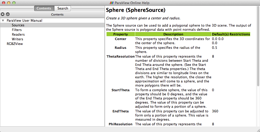
Regardless of whether the GUI contains a custom panel for a pipeline object, you can still get information about that object’s properties from the GUI’s online help. As always, bring up the help with the toolbar button. You can find documentation for all the available pipeline objects under the Sources, Filters, Readers, and Writers entries in the help Contents. Each entry gives a list of objects of that type. Clicking on any one of the objects gives a list of the properties you can set from within Python.

3.7. Reading from Files

The equivalent to opening a file in the ParaView GUI is to create a reader in Python scripting. Reader objects are created in much the same way as sources and filters; paraview.simple has a function for each reader type that creates the pipeline object and returns a proxy object. One can instantiate any given reader directly as described below, or more simply call reader = OpenDataFile({filename})

All reader objects have at least one property (hidden in the GUI) that specifies the file name. This property is conventionally called either FileName or FileNames. You should always specify a valid file name when creating a reader by placing something like FileName={full path} in the arguments of the construction object. Readers often do not initialize correctly if not given a valid file name.

Exercise 3.8 (Creating a Reader)

We are going to start a fresh visualization, so if you have been following along with the exercises so far, now is a good time to reset ParaView. The easiest way to do this is to select from the toolbar. You will also need the Python shell. If you have not already done so, open it with View → Python Shell from the menu.

In this exercise we are loading the disk_out_ref.ex2 file from the Python shell. Locate this file on your computer and be ready to type or copy it into the Python shell. We will reference it as {path}/disk_out_ref.ex2. You can use the file browser to help you locate this file. (Click on the Examples quick access directory and observe where the file browser takes you.) Common paths for the file are as follows:

Mac

/Applications/ParaView-x.x.x.app/Contents/examples

Windows

C:/Program Files/ParaView x.x.x/examples

Linux

/usr/local/lib/paraview-x.x.x/examples

Create the reader while specifying the file name by entering the following in the Python shell.

reader = OpenDataFile('{path}/disk_out_ref.ex2')
Show()
Render()
ResetCamera()

3.8. Querying Field Attributes

In addition to having properties specific to the class, all proxies for pipeline objects share a set of common properties and methods. Two very important such properties are the PointData and CellData properties. These properties act like dictionaries, an associative array type in Python, that maps variable names (in strings) to ArrayInformation objects that hold some characteristics of the fields. Of particular note are the ArrayInformation methods GetName, which returns the name of the field, GetNumberOfComponents, which returns the size of each field value (1 for scalars, more for vectors), and GetRange, which returns the minimum and maximum values for a particular component.

Exercise 3.9 (Getting Field Information)

This exercise is a continuation of Exercise 3.8. You will need to finish that exercise before beginning this one.

To start with, get a handle to the point data and print out all of the point fields available.

pd = reader.PointData
print(pd.keys())

Get some information about the “pres” and “v” fields.

print(pd["pres"].GetNumberOfComponents())
print(pd["pres"].GetRange())
print(pd["v"].GetNumberOfComponents())

Now let us get fancy. Use the Python for construct to iterate over all of the arrays and print the ranges for all the components.

for ai in pd.values():
   print(ai.GetName(), ai.GetNumberOfComponents(), end=" ")
   for i in range(ai.GetNumberOfComponents()):
      print(ai.GetRange(i), end=" ")
   print()

3.9. Representations

Representations are the “glue” between the data in a pipeline object and a view. The representation is responsible for managing how a dataset is drawn in the view. The representation defines and manages the underlying rendering objects used to draw the data as well as other rendering properties such as coloring and lighting. Parameters made available in the Display group of the GUI are managed by representations. There is a separate representation object instance for every pipeline-object–view pair. This is so that each view can display the data differently.

Representations are created automatically by the GUI. In python scripting they are created with the Show function instead. In fact Show returns a proxy to the representation. Therefore you can save Show’s return value in a variable as we’ve done above for sources, filters and readers. If you neglect to save it, you can always get it back with the GetRepresentation function. With no arguments, this function will return the representation for the active pipeline object and the active view. You can also specify a pipeline object or view or both.

Exercise 3.10 (Coloring Data)

This exercise is a continuation of Exercise 3.8 (and optionally Exercise 3.9). If you do not have the exodus file open, you will need to finish Exercise 3.8 before beginning this one.

Let us change the color of the geometry to blue and give it a very pronounced specular highlight (that is, make it really shiny). Type in the following into the Python shell to get the representation and change the material properties.

readerRep = GetRepresentation()
readerRep.DiffuseColor = [0, 0, 1]
readerRep.SpecularColor = [1, 1, 1]
readerRep.SpecularPower = 128
readerRep.Specular = 1
Render()

Now rotate the camera with the mouse in the GUI to see the effect of the specular highlighting.

We can also use the representation to color by a field variable. There is actually quite a bit of state that must be set to change field variables. The ColorBy function provides a simple interface to color a mesh by a field value. A subsequent call to UpdateScalarBars also updates the color bar annotation. Enter the following into the Python shell to color the mesh by the “pres” field variable.

ColorBy(readerRep, ("POINTS", "pres"))
UpdateScalarBars()
Render()

3.10. Views

Drawing areas or windows are called Views in ParaView. As with readers, sources, filters, and representations, views are wrapped into python objects and these can be created, obtained and controlled via scripts.

Views are usually created for you by the GUI, but in python you have to create views more intentionally. The most convenient way to do so is to rely on the way that Render returns a view, creating one first if necessary. If you prefer, you can create specific view types via CreateView(’{viewname}’) or CreateRenderView, CreateXYPlotView and the like. However you make them, call GetRenderViews to get a list of all Views, or GetActiveView get access to the currently active view. There is also a function named GetRenderView (no ‘s’ on the end) that gets the active view if there is one or creates a new one if there is no active view.

Once you have a view you have access to all of the properties that you see on the View group of the GUI. For instance you can easily turn on and off the orientation widget, change the background color, alter the lighting and more. Besides these first level properties, the view also gives you access to other scene wide controls such as the camera, animation time, and when not running alongside the GUI, the view’s size.

Exercise 3.11 (Controlling the View)

This exercise is a continuation of Exercise 3.8 (and optionally Exercise 3.9, and Exercise 3.10. If you do not have the exodus file open, you will need to finish Exercise 3.8 before beginning this one.

Let us change the background color of the scene from ParaView’s default gray to a nice gradient instead. Type the following into the Python shell to get a hold of the View and change it.

view = GetActiveView()
view.Background = [0, 0, 0]
view.Background2 = [0, 0, 0.6]
view.UseGradientBackground = True
Render()

Next, let us ask the view what position the camera is sitting at, and then move it within a for loop to create a short animation.

x, y, z = view.CameraPosition
print(x, y, z)
for iter in range(0,10):
   x = x + 1
   y = y + 1
   z = z + 1
   view.CameraPosition = [x, y, z]
   print(x, y, z)
   Render()

3.11. Saving Results

Within a script it is easy to save out results, and by saving your data and your scripts it becomes easy to create reproducible visualization with ParaView.

As within the GUI, there are several products that you might like to save out when you are working with ParaView.

To save out the data produced by a filter, add a writer to the filter with the desired filename using the CreateWriter function and then update the writer proxy with the UpdatePipeline method. This is analogous to clicking on a pipeline element and selecting File → Save Data.
Saving images is as simple as typing SaveScreenshot(’{path}/filename.still_extension’).
Assuming your ParaView is linked to an encoder and codecs, saving compressed animations is as simple as typing WriteAnimation(’{path}/filename.animation_extension’).

In all cases ParaView uses the file name extension to determine the specific file type to create.

Exercise 3.12 (Save Results)

This exercise is a continuation of Exercise 3.8 (and optionally Exercise 3.9 through Exercise 3.11). If you do not have the exodus file open, you will need to finish Exercise 3.8 before beginning this one.

Let us first probe the data to get something compact out of it. Then we will save out the result of the probe in the form of a comma separated values file so that we can look at it in a text editor and import it into any other tool we choose.

plot = PlotOverLine()
plot.Source.Point1 = [0, 0, 0]
plot.Source.Point2 = [0, 0, 10]
writer = CreateWriter("{path}/plot.csv")
writer.UpdatePipeline()

Next, lets create a LineChartView to show the plot in and then save out a screenshot of our results.

plotView = FindViewOrCreate("MyView", viewtype="XYChartView")
Show(plot)
Render()
SaveScreenshot("{path}/plot.png")

As you can see, ParaView’s scripting interface is quite powerful, and once you know the fundamentals and are familiar with Python’s syntax, it is fairly easy to get up and running with it. We have just touched on the higher level aspects of ParaView scriptability in this tutorial. More details, including how to run python scripted filters, how to work with numpy and other tools, and how to package your scripts for execution under batch schedulers can be found online.