8. Remote and parallel visualization
One of the goals of the ParaView application is enabling data analysis and visualization for large datasets. ParaView was born out of the need for visualizing simulation results from simulations run on supercomputing resources that are often too big for a single desktop machine to handle. To enable interactive visualization of such datasets, ParaView uses remote and/or parallel data processing. The basic concept is that if a dataset cannot fit on a desktop machine due to memory or other limitations, we can split the dataset among a cluster of machines, driven from your desktop. In this chapter, we will look at the basics of remote and parallel data processing using ParaView. For information on setting up clusters, please refer to the ParaView Wiki [ThePCommunity].
Did you know?
Remote and parallel processing are often used together, but they refer to different concepts, and it is possible to have one without the other.
In the case of ParaView, remote processing refers to the concept of
having a client, typically paraview or pvpython, connecting to a pvserver, which
could be running on a different, remote machine. All the data
processing and, potentially, the rendering can happen on the
pvserver. The client drives the visualization process by
building the visualization pipeline and viewing the generated results.
Parallel processing refers to a concept where instead of single core
— which we call a rank — processing the entire dataset, we
split the dataset among multiple ranks. Typically, an instance of
pvserver runs in parallel on more than one rank. If a
client is connected to a server that runs in parallel, we are using
both remote and parallel processing.
In the case of pvbatch, we have an application that operates in parallel
but without a client connection. This is a case of parallel
processing without remote processing.
8.1. Understanding remote processing
Let’s consider a simple use-case. Let’s say you have two computers, one located
at your office and another in your home. The one at the office is a nicer,
beefier machine with larger memory and computing capabilities than the one at
home. That being the case, you often run your simulations on the office
machine, storing the resulting files on the disk attached to your office
machine. When you’re at work, to visualize those results, you simply launch
paraview and open the data file(s). Now, what if you need to
do the visualization and data analysis from home? You have several options:
You can copy the data files over to your home machine and then use
paraviewto visualize them. This is tedious, however, as you not only have to constantly keep copying/updating your files manually, but your machine has poorer performance due to the decreased compute capabilities and memory available on it!You can use a desktop sharing system like Remote Desktop or VNC, but those can be flaky depending on your network connection.
Alternatively, you can use ParaView’s remote processing capabilities. The
concept is fairly simple. You have two separate processes: pvserver (which runs
on your work machine) and a paraview client (which runs on your home machine).
They communicate with each other over sockets (over an SSH tunnel, if needed).
As far as using paraview in this mode, it’s no different than how we have been
using it so far – you create pipelines and then look at the data produced by
those pipelines in views and so on. The pipelines themselves, however, are created
remotely on the pvserver process. Thus, the pipelines have access to the disks
on your work machine. The Open File dialog will in fact browse the file
system on your work machine, i.e., the machine on which pvserver is running. Any
filters that you create in your visualization pipeline execute on the
pvserver.
While all the data processing happens on the pvserver, when it
comes to rendering, paraview can be configured to either do the rendering on
the server process and deliver only images to the client (remote rendering)
or to deliver the geometries to be rendered to the client and let it do the
rendering locally (local rendering).
When remote rendering, you’ll be using the graphics capabilities on your work
machine (the machine running the pvserver). Every time a new rendering needs to
be obtained (for example, when pipeline parameters are changed or you interact
with the camera, etc.), the pvserver process will re-render a new image and
deliver that to the client. When local rendering, the geometries to be rendered
are delivered to the client and the client renders those locally. Thus, not all
interactions require server-side processing. Only when the
visualization pipeline is updated does the server need to deliver
updated geometries to the client.
8.2. Remote visualization in paraview
8.2.1. Starting a remote server
To begin using ParaView for remote data processing and visualization, we must
first start the server application pvserver on the remote system. To do this,
connect to your remote system using a shell and run:
> pvserver
You will see this startup message on the terminal:
Waiting for client...
Connection URL: cs://myhost:11111
Accepting connection(s): myhost:11111
This means that the server has started and is listening for a connection from a client.
8.2.2. Configuring a server connection
To connect to this server with the
paraview client, select File > Connect or click
the  icon in the toolbar to bring up the
Choose Server Configuration dialog.
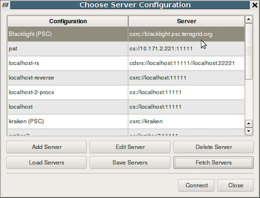
Fig. 8.12 The Choose Server Configuration dialog is used to connect to a server.
Common Errors
If your server is behind a firewall and you are attempting to connect to it from outside the firewall, the connection may not be established successfully. You may also try reverse connections ( Section 8.4) as a workaround for firewalls. Please consult your network manager if you have network connection problems.
Figure Fig. 8.12 shows the Choose Server
Configuration dialog with a number of entries for remote servers. In
the figure, a number of servers have already been configured, but when
you first open this dialog, this list will be empty. Before you can
connect to a remote server, you will need to add an entry to the list
by clicking on the Add Server button. When you do, you will see
the Edit Server Configuration dialog as in
Figure Fig. 8.13.
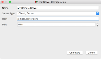
Fig. 8.13 The Edit Server Configuration dialog is used to
configure settings for connecting to remote servers.
You will need to set a name for the connection, the server type, the
DNS name of the host on which you just started the server, and the
port. The default Server Type is set to Client / Server, which
means that the server will be listening for an incoming connection
from the client. There are several other options for this setting that
we will discuss later.
When you are done, click the Configure button. Another dialog, as
shown in Fig. 8.14, will appear
where you specify how to start the server. Since we started the server
manually, we will leave the Startup Type on the default
Manual setting. You can optionally set the Startup Type to
Command and specify an external shell command to launch a server
process.
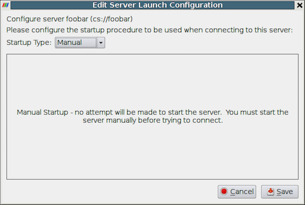
Fig. 8.14 Configure the server manually. It must be started outside of ParaView.
When you click the Save button, this particular server
configuration will be saved for future use. You can go back and edit
the server configuration by selecting the entry in the list of servers
and clicking the Edit Server button in the Choose Server
Configuration dialog. You can delete it by clicking the Delete
button.
Server configurations can be imported and exported through the
Choose Server
Configuration
dialog. Use the Load Servers
button to load a server configuration file and the Save Servers
button to save a server configuration file. Files can be exchanged
with others to access the same remote servers.
Did you know?
Visualization centers can provide system-wide server configurations on
web servers to allow non-experts to simply select an already
configured ParaView server. These site-wide settings can be
loaded with the Fetch Servers button. Advanced users may also want
to specify their own servers in more details.
These features are provided thanks to ParaView Server Configuration files
(Section 8.5).
8.2.3. Connect to the remote server
To connect to the server, select the server configuration you just set
up from the configuration list, modify the timeout in the timeout combo
box if needed and click Connect. ParaView will try to connect to
the server until it succeed or timeout is reached. In that case, you can just
retry as needed. Once the connection steps succeed, we are now connected and
ready to build the visualization pipelines.
Common Errors
ParaView does not perform any kind of authentication when clients
attempt to connect to a server. For that reason, we recommend that you
do not run pvserver on a computing resource that is open to the outside
world.
ParaView also does not encrypt data sent between the client and server. If your data is sensitive, please ensure that proper network security measures have been taken. The typical approach is to use an SSH tunnel within your server configuration files using native SSH support (Section 8.5.16).
8.2.4. Managing multiple clients
pvserver can be configured to accept connections from multiple clients at the same time.
In this case only one, called the master, can interact with the pipeline.
Others clients are only allowed to visualize the data. The Collaboration Panel
shares information between connected clients.
To enable this mode, pvserver must be started with the --multi-clients flag:
pvserver --multi-clients
If your remote server is accessible from many users, you may want to restrict the access.
This can be done with a connect id.
If your client does not have the same connect-id as the server you want to connect to,
you will be prompted for a connect-id.
Then, if you are the master, you can change the connect-id in the Collaboration Panel.
Note that initial value for connect-id can be set by starting the pvserver
(and respectively paraview) with the --connect-id flag, for instance:
pvserver --connect-id=147
The master client can also disable further connections in the Collaboration Panel
so you can work alone, for instance. Once you are ready, you may allow other people to connect
to the pvserver to share a visualization. This is the default feature when pvserver is
started with --multi-clients --disable-further-connections.
8.2.5. Setting up a client/server visualization pipeline
Using paraview when connected to a remote server is not any different than when
it’s being used in the default stand-alone mode. The only difference, as far as
the user interface goes, is that the Pipeline Browser reflects the name of
the server to which you are connected. The address of the server connection next to
the  icon changes from
 builtin
to cs://myhost:11111 .
Since the data processing pipelines are executing on the server side, all file
I/O also happens on the server side. Hence, the Open File dialog, when
opening a new data file, will browse the file system local to the pvserver
executable and not the paraview client.
8.3. Remote visualization in pvpython
The pvpython executable can be used by itself for visualization of local
data, but it can also act as a client that connects to a remote pvserver.
Before creating a pipeline in pvpython, use the Connect function:
# Connect to remote server "myhost" on the default port, 11111
>>> Connect("myhost") # Connect to remote server "myhost" on a
                      # specified port
>>> Connect("myhost", 11111)
Now, when new sources are created, the data produced by the sources
will reside on the server. In the case of pvpython, all data remains on
the server and images are generated on the server too. Images are
sent to the client for display or for saving to the local filesystem.
8.4. Reverse connections
It is frequently the case that remote computing resources are located behind a network firewall, making it difficult to connect a client outside the firewall to a server behind it. ParaView provides a way to set up a reverse connection that reverses the usual client server roles when establishing a connection.
To use a remote connection, two steps must be performed. First,
in paraview, a new connection must be configured with the connection type
set to reverse. To do this, open the Choose Server Configuration
dialog through the File > Connect menu item. Add a new
connection, setting the Name to myhost (reverse)'', and select
``Client / Server (reverse connection) for Server Type . Click
Configure . In the Edit Server Launch Configuration dialog that
comes up, set the Startup Type to Manual . Save the
configuration. Next, select this configuration and click Connect .
A message window will appear showing that the client is awaiting a
connection from the server.
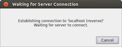
Fig. 8.15 Message window showing that the client is awaiting a connection from a server.
Second, pvserver must be started with the --reverse-connection
(-rc) flag. To tell pvserver the name of the client, set
the --client-host (-ch) command-line argument to the
hostname of the machine on which the paraview client is running. You
can specify a port with the --server-port (-sp)
command-line argument.
pvserver -rc --client-host=mylocalhost --server-port=11111
When the server starts, it prints a message indicating the success or failure of connecting to the client. When the connection is successful, you will see the following text in the shell:
Connecting to client (reverse connection requested)...
Connection URL: csrc://mylocalhost:11111
Client connected.
Did you know?
Most connection related command line option can be set using a server settings file, as described in this section: Section 14.3.2
To wait for reverse connections from a pvserver in pvpython, you use
ReverseConnect instead of Connect .
# To wait for connections from a 'pvserver' on the default port 11111
>>> ReverseConnect()

# Optionally, you can specify the port number as the argument.
>>> ReverseConnect(11111)
8.5. ParaView Server Configuration Files
In the Choose Server Configuration dialog, it is possible
to Load Servers and Save Servers using the dedicated buttons.
Server configurations are stored in ParView Server Configuration files (.pvsc).
These files make it possible to extensively customize the server connection process. During startup, ParaView looks at several locations for server configurations to load by default.
- On Unix-based systems and macOS
default_servers.pvscin the ParaView executable directory (you can do als -l /proc/<paraview PID here>/exeto identify the executable directory)under each of
XDG_DATA_DIRS, looking forParaView/servers.pvsc./usr/local/share/ParaView/servers.pvscor/usr/share/ParaView/servers.pvsc$HOME/.config/ParaView/servers.pvsc(ParaView will save user defined servers here)
- On Windows
default_servers.pvscin the ParaView executable directory%COMMON_APPDATA%\ParaView\servers.pvsc%APPDATA%\ParaView\servers.pvsc(ParaView will save user defined servers here)
The exact procedure to find the writable directory is detailed in Section 14.4.
Here are a few examples of some common use-cases.
8.5.1. Case One: Simple command server startup
In this use-case, we are connecting to a locally started pvserver (localhost) on the 11111 port,
except that the command to start the server will be automatically called just before connecting to the server,
we will wait for timeout seconds before aborting the connection.
<Server name="case01" resource="cs://localhost:11111" timeout="10">
  <CommandStartup>
    <Command process_wait="0" delay="5" exec="/path/to/pvserver"/>
  </CommandStartup>
</Server>
Here, CommandStartup element specify that a command will be run before connecting to the server.
The Command element contains the details about this command, which includes
process_wait, the time in seconds that paraview will wait for the process to start,
delay, the time in seconds paraview will wait after running the command to try to connect and finally,
exec, which is the command that will be run and usually contains the path to pvserver but could also
contain a mpi command to start pvserver distributed or to any script or executable on the localhost
filesystem.
8.5.2. Case Two: Simple remote server connection
In this use-case, we are setting a configuration for a simple server connection (to a pvserver processes) running on a node named “amber1”, at port 20234.
The pvserver process will be started manually by the user.
<Server name="case02" resource="cs://amber1:20234">
  <ManualStartup/>
</Server>
Here, name specify the name of the server as it will appear in the pipeline browser, resource identifies the type if the connection (cs – implying client-server), host name and port.
If the port number i.e. :20234 part is not specified in the resource, then the default port number (which is 11111) is assumed. Since the user starts pvserver processes manually, we use ManualStartup.
8.5.3. Case Three: Server connection with user-specified port
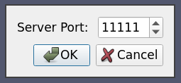
This is the same as case two except that we want to ask the user each time the port number to connect to the pvserver at.
<Server name="case03" resource="cs://amber1">
  <ManualStartup>
    <Options>
      <Option name="PV_SERVER_PORT" label="Server Port: ">
        <Range type="int" min="1" max="65535" step="1" default="11111" />
      </Option>
    </Options>
  </ManualStartup>
</Server>
Here the only difference is the Options element.
This element is used to specify run-time options that the user specifies when connecting to the server, see this section for a list of available run-time options.
In this case, we want to show the user an integral spin-box to select the port number, hence we use the Range element to specify the type of the option.
When the user connects to this server, he is shown a dialog similarly to the following image:
8.5.4. Case Four: Simple connection to a data-server/render-server
This is the same as case two, except that instead of a single server (i.e. pvserver),
we are connecting to a separate render-server/data-server with pvdataserver running on port 20230 on amber1 and pvrenderserver running port 20233 on node amber2.
<Server name="case04" resource="cdsrs://amber1:20230//amber2:20233">
  <ManualStartup />
</Server>
The only difference with case two, is the resource specification. cdsrs indicates that it is a client-dataserver-renderserver configuration.
The first host:port pair is the dataserver while the second one is the render server.
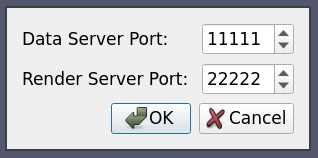
8.5.5. Case Five: Connection to a data-server/render-server with user specified server port
This is a combination of case three and case four, where we want to ask the user for the port number for both the render server and the data server.
<Server name="case05" resource="cdsrs://localhost//localhost">
  <ManualStartup>
    <Options>
      <Option name="PV_DATA_SERVER_PORT" label="Data Server Port: ">
        <Range type="int" min="1" max="65535" step="1" default="11111" />
      </Option>
      <Option name="PV_RENDER_SERVER_PORT" label="Render Server Port: ">
        <Range type="int" min="1" max="65535" step="1" default="22222" />
      </Option>
    </Options>
  </ManualStartup>
</Server>
The XML is quite self-explanatory given what we has already been explained above. The options dialog produced by this XML looks as follows:
8.5.6. Case Six: Reverse Connection
By default the client connects to the server processes. However it is possible to tell the paraview client to wait for the server to connect to it instead.
This is called a reverse connection. In such a case the server processes must be started with --reverse-connection or --rc flag.
To indicate reverse connection in the server configuration xml, the only change is suffixing the resource protocol part with rc (for reverse connection). eg.
resource="csrc://localhost" -- connect to pvserver on localhost using reverse connection
resource="cdsrsrc://localhost//localhost" -- connect to pvdataserver/pvrenderserver using reverse connection.
So a simple local reverse connection server configuration, similarly to case one, would look like this
<Server name="case06" resource="csrc://localhost:11111">
  <CommandStartup>
    <Command exec="/path/to/pvserver --reverse-connection --client-host=localhost"/>
  </CommandStartup>
</Server>
Here the --client-host=localhost in the exec is actually not needed has this is the default.
8.5.7. Case Seven: Server command with option
As we have seen in case one, the server can be started by ParaView on connection, but this can be combined with the Option element
as seen in case three to create a dynamically generated server command.
<Server name="case07" resource="cs://localhost">
  <CommandStartup>
    <Options>
      <!-- The user chooses the port on which to start the server -->
      <Option name="PV_SERVER_PORT" label="Server Port: ">
        <Range type="int" min="1" max="65535" step="1" default="11111" />
      </Option>
    </Options>
    <Command delay="5" exec="/path/to/pvserver">
      <Arguments>
        <Argument value="--server-port=$PV_SERVER_PORT$" />
      </Arguments>
    </Command>
  </CommandStartup>
</Server>
As with case one, we are using CommandStartup and Command elements.
Command line arguments can be passed to the command executed using the Arguments element.
All runtime environment variables specified as $name$ are replaced with the actual values.
Eg. in this case $PV_SERVER_PORT$ gets replaced by the port number chosen by the user in the options dialog.
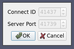
8.5.8. Case Eight: Using connection-id and random port
In many cases, a server cluster may be running multiple pvserver (or pvdataserver/pvrenderserver) processes for different users.
In that case we need some level of authentication between the server and the client.
This can be achieved (at a very basic level) with the connect-id option.
If specified on the command line when starting the server processes (using --connect-id) then the server will allow only that client which reports the same connection id to connect.
We also want to avoid port collision with other users, so we use a random port for the server connection.
Here is an example similarly to case seven but with a connect-id option and random server port.
<Server name="case08" resource="cs://localhost">
  <CommandStartup>
    <Options>
      <Option name="PV_CONNECT_ID" label="Connect ID" readonly="true">
        <Range type="int" min="1" max="65535" default="random" />
      </Option>
      <Option name="PV_SERVER_PORT" label="Server Port" readonly="true">
        <Range type="int" min="11111" max="65535" default="random" />
      </Option>
    </Options>
    <Command exec="/path/to/pvserver" delay="5">
      <Arguments>
        <Argument value="--connect-id=$PV_CONNECT_ID$" />
        <Argument value="--server-port=$PV_SERVER_PORT$" />
      </Arguments>
    </Command>
  </CommandStartup>
</Server>
In this case, the readonly attribute on the Option indicates that the value cannot be changed by the user, it is only shown for information purposes.
The default value for the PV_CONNECT_ID and PV_SERVER_PORT is set to random so that ParaView makes up a value at run time.
Of course, in a production environment they should be assigned by user instead of randomly generated.
8.5.9. Case Nine: Starting server using ssh
In this use case the server process is spawned on some remote host using specifically crafted ssh command. We want the user to be able to specify the ssh executable. We also want to preserve the ssh executable path across ParaView sessions so that the user does not have to enter it each time.
<Server name="case09" resource="cs://localhost:11111">
  <CommandStartup>
    <Options>
      <Option name="SSH_USER" label="SSH Username" save="true">
        <!-- choose the username. Since 'save' is true, this value will
             be maintained across sessions -->
        <String default="user" />
      </Option>
      <Option name="SSH_EXE" label="SSH Executable" save="true">
        <!-- select the SSH executable. Since 'save' is true, this value will
             also be maintinaed across sessions -->
        <File default="ssh" />
      </Option>
    </Options>
    <Command exec="$SSH_EXE$" delay="5">
      <Arguments>
        <Argument value="-L8080:amber5:11111" /> <!-- port forwarding -->
        <Argument value="amber5" />
        <Argument value="-l" />
        <Argument value="$SSH_USER$" />
        <Argument value="/path/to/pvserver" />
      </Arguments>
    </Command>
  </CommandStartup>
</Server>
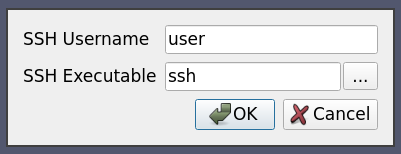
Note here that the value for the exec attribute is set to $SSH_EXE$ hence it gets replaced by the user selected ssh executable.
We use the optional attribute save on the Option element to tell ParaView to preserve the user chosen value across ParaView sessions
so that the user doesn’t have to enter the username and the ssh executable every time he wants to connect to this server.
Did you know?
While SSH connection can be started by crafting the command, ParaView
now support SSH connection natively by specifying a SSHCommand, see below
for more information.
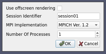
8.5.10. Case Ten: Starting server using custom script with custom user-settable options
This example will illustrate the full capability of server configuration. Suppose we have a custom script “MyServerStarter” that takes in multiple arguments to start the server process. We want the user to be able to set up values for these arguments when he tries to connect to using this configuration. As an example, let’s say MyServerStarter takes the following arguments:
--force-offscreen-rendering– to indicate use of offscreen rendering
--force-onscreen-rendering– to indicate on-screen rendering (this can be assumed from absence of--force-offscreen-rendering, but we are using it as an example)
--session-name=<string>– some string identifying the session
--mpitype=<mpich1.2|mpich2|openmpi>– choose between available MPI implementations
--num-procs=<num>– number of server processes
--server-port– port number passed the pvserver processes
All (except the –server-port) of these must be settable by the user at the connection time. This can be achieved as follows:
<Server name="case10" resource="cs://localhost">
  <CommandStartup>
    <Options>
      <Option name="OFFSCREEN" label="Use offscreen rendering">
        <Boolean true="--use-offscreen" false="--use-onscreen" default="false" />
      </Option>
      <Option name="SESSIONID" label="Session Identifier">
        <String default="session01"/>
      </Option>
      <Option name="MPITYPE" label="MPI Implementation">
        <Enumeration default="mpich1.2">
          <Entry value="mpich1.2" label="MPICH Ver. 1.2" />
          <Entry value="mpich2" label="MPICH Ver 2.0" />
          <Entry value="openmpi" label="Open MPI" />
        </Enumeration>
      </Option>
      <Option name="NUMPROC" label="Number Of Processes">
        <Range type="int" min="1" max="256" step="4" default="1" />
      </Option>
    </Options>
    <Command exec="/path/to/MyServerStarter" delay="5">
      <Arguments>
        <Argument value="--server-port=$PV_SERVER_PORT$" />
        <Argument value="--mpitype=$MPITYPE$" />
        <Argument value="--num-procs=$NUMPROC$" />
        <Argument value="$OFFSCREEN$" />
        <Argument value="--session-name=$SESSIONID$" />
      </Arguments>
    </Command>
  </CommandStartup>
</Server>
Each Option defines a new run-time variable that can be accessed as ${name}$ in the Command section.
When the user tries to connect using this configuration, he is shown the following options dialog:
This can be extended to start the server processes using ssh or any batch scheduler etc. as may be the required by the server administrator. This can also be set up to use reverse connection (by changing the protocol in the resource attribute).
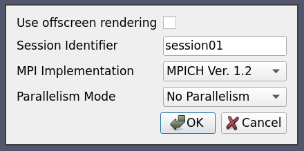
8.5.11. Case Eleven: Case Ten + Switch Statement
This is same as case ten with one change: We no longer allow the user to choose the number of processes. Instead, the number of processes is automatically selected based on the value of the distribution combobox.
<Server name="case11" resource="cs://localhost">
  <CommandStartup>
    <Options>
      <Option name="OFFSCREEN" label="Use offscreen rendering">
        <Boolean true="--use-offscreen" false="--use-onscreen" default="false" />
      </Option>
      <Option name="SESSIONID" label="Session Identifier">
        <String default="session01"/>
      </Option>
      <Option name="MPITYPE" label="MPI Implementation">
        <Enumeration default="mpich1.2">
          <Entry value="mpich1.2" label="MPICH Ver. 1.2" />
          <Entry value="mpich2" label="MPICH Ver 2.0" />
          <Entry value="openmpi" label="Open MPI" />
        </Enumeration>
      </Option>
      <Option name="DISTRIBUTION" label="Distribution Mode">
        <Enumeration default="notDistributed">
          <Entry value="notDistributed" label="Not Distributed" />
          <Entry value="someDistribution" label="Some Distribution" />
          <Entry value="highDistribution" label="Highly Distributed" />
        </Enumeration>
      </Option>
      <Switch name="DISTRIBUTION">
        <Case value="notDistributed">
          <Set name="NUMPROC" value="1" />
        </Case>
        <Case value="someDistribution">
          <Set name="NUMPROC" value="2" />
        </Case>
        <Case value="highDistribution">
          <Set name="NUMPROC" value="10" />
        </Case>
      </Switch>
    </Options>
    <Command exec="/path/to/MyServerStarter" delay="5">
      <Arguments>
        <Argument value="--server-port=$PV_SERVER_PORT$" />
        <Argument value="--mpitype=$MPITYPE$" />
        <Argument value="--num-procs=$NUMPROC$" />
        <Argument value="$OFFSCREEN$" />
        <Argument value="--session-name=$SESSIONID$" />
      </Arguments>
    </Command>
  </CommandStartup>
</Server>
The Switch statement can only have Case statements as children, while the Case statement can only have Set statements as children.
Set statements are not much different from Option except that the value is fixed and the user is not prompted to set that value.
8.5.12. Case Twelve: Simple SSH run server command
If Command element let you craft SSH commands, it can be quite complex to do so and the pipeline
browser in ParaView may not show the correct server as it could connect through a ssh tunnel.
Here, similarly to case one, we use native ssh support to start a pvserver process remotely, on amber1, before connecting to it directly on the default port:
<Server name="case12" resource="cs://amber1">
  <CommandStartup>
    <SSHCommand exec="/path/to/pvserver" delay="5">
      <SSHConfig user="user"/>
    </SSHCommand>
  </CommandStartup>
</Server>
First SSHCommand element is used instead of Command so that ParaView knows to use native ssh support.
Then the SSHConfig element is used to configure the ssh connection. The user attribute is the SSH user to use with SSH.
If a password is needed, it will be asked on the terminal used to run ParaView, which may not be visible in certain cases.
8.5.13. Case Thirteen: SSH run server command with complex config
Here, similarly to case twelve, we use native ssh support to start a pvserver process remotely, on amber1, before connecting to it directly, but we specify much more specifically the configuration to use.
<Server name="case13" resource="cs://amber1">
  <CommandStartup>
    <Options>
      <!-- The user chooses the port on which to start the server -->
      <Option name="PV_SERVER_PORT" label="Server Port: ">
        <Range type="int" min="1" max="65535" step="1" default="11111" />
      </Option>
    </Options>
    <SSHCommand exec="/path/to/pvserver" delay="5">
      <SSHConfig user="user" port="2222">
        <Terminal exec="/usr/bin/xterm"/>
        <SSH exec="/usr/bin/ssh"/>
      </SSHConfig>
      <Arguments>
        <Argument value="--server-port=$PV_SERVER_PORT$"/>
      </Arguments>
    </SSHCommand>
  </CommandStartup>
</Server>
Inside the SSHConfig element, we use different elements.
First, we added a port attribute to specify which port to use, using the -p option of the SSH command.
Here, Terminal element is used to specify that ParaView will try to open a terminal to ask the
user for his password. Here, the terminal executable is specified using the exec attribute.
If it was not, ParaView would try to find one automatically (Linux and Windows).
On Linux and macOS, it is possible to specify the command_option to use with the terminal executable.
This is needed when using gnome-terminal, eg: <Terminal exec="/usr/bin/gnome-terminal" command_option="--"/>
When troubleshooting server configuration, not using Terminal element is suggested
as the terminal will close as soon as the command finish executing.
On Linux, it is also possible to replace the Terminal element by the AskPass element
to specify the ParaView should use SSH_ASKPASS so that a ask-pass binary is used when asking
for the SSH password.
Finally, the SSH element specify the SSH binary to use thanks to its exec attribute.
We also use PV_SERVER_PORT, similarly to case seven to let the user select the port to connect to.
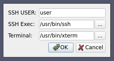
8.5.14. Case Fourteen: SSH run server command with user chosen config
Here, similarly to case thirteen and five, we use native ssh support to start a pvserver process remotely, on amber1, before connecting to it directly, but we let the user choose interactively some SSH options.
<Server name="case14" resource="cs://amber1">
  <CommandStartup>
    <Options>
      <Option label="SSH USER:" name="SSH_USER" save="true">
        <String default="user"/>
      </Option>
      <Option label="SSH Exec:" name="SSH_EXEC" save="true">
        <File default="/usr/bin/ssh" />
      </Option>
      <Option label="Terminal:" name="TERMINAL" save="true">
        <File default="/usr/bin/xterm"/>
      </Option>
    </Options>
    <SSHCommand exec="/path/to/pvserver" delay="5">
      <SSHConfig user="$SSH_USER$">
        <Terminal exec="$TERMINAL$"/>
        <SSH exec="$SSH_EXEC$"/>
      </SSHConfig>
      <Arguments>
        <Argument value="--server-port=$PV_SERVER_PORT$"/>
      </Arguments>
    </SSHCommand>
  </CommandStartup>
</Server>
Similarly to all other options, SSH related options can be set interactively by the user. Here we let the user set the SSH user, the SSH executable as well as the Terminal executable to use when connecting through ssh.
8.5.15. Case Fifteen: Ssh run server command with reverse connection
Similarly to case twelve and thirteen, we use native ssh support to start a reverse connection pvserver process remotely, on amber1, before letting it connect to ParaView using the hostname of the client on static non-default port.
<Server name="case15" resource="csrc://amber1:11112">
  <CommandStartup>
    <SSHCommand exec="/path/to/pvserver" delay="5">
      <SSHConfig user="user">
        <Terminal/>
      </SSHConfig>
      <Arguments>
        <Argument value="--reverse-connection"/>
        <Argument value="--client-host=$PV_CLIENT_HOST$"/>
        <Argument value="--server-port=$PV_SERVER_PORT$"/>
      </Arguments>
    </SSHCommand>
  </CommandStartup>
</Server>
The only difference with case twelve is in the resource, which now contain the reverse connection
as well as the usage of $PV_CLIENT_HOST$ in the arguments for the reverse connection,
automatically set to the hostname of the client which the server should be able to resolve to an ip
to connect to.
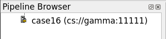
8.5.16. Case Sixteen: Secured Connection to a Server through SSH tunnel
To communicate securely through a ssh tunnel, something usually done with a crafted command looking like this:
ssh -L local_port:localhost:server_port user@remote /path/to/pvserver --server-port server_port
You would then connect on a server on localhost:local_port within ParaView.
This is complex to set up either manually of with a Command element. Also,
the true server and port will not appear in the pipeline browser in ParaView.
This is however natively supported with SSHCommand element.
Here we create a secured SSH tunnel to amber1 before connecting through the SSH tunnel on
the 11111 port, the local ParaView client internally uses the 8080 port.
<Server name="case16" resource="cs://amber1:11111">
  <CommandStartup>
    <SSHCommand exec="/path/to/pvserver" delay="5">
      <SSHConfig user="user">
        <Terminal/>
        <PortForwarding local="8080"/>
      </SSHConfig>
      <Arguments>
        <Argument value="--server-port=$PV_SERVER_PORT$"/>
      </Arguments>
    </SSHCommand>
  </CommandStartup>
</Server>
Similarly to case thirteen, we only add a PortForwarding element in the SSHConfig element with the optional local attribute port,
so that ParaView creates a SSH tunnel to connect through.
If local attribute is not specified, the server port will be used.
The $PV_SERVER_PORT$ is automatically set to the value of the port to use within the SSH tunnel.
In ParaView, the tunnel will be integrated nicely in the UI with the correct port and hostname in the pipeline browser,
the server icon will look different with a small lock to note the secured nature of this connection:
8.5.17. Case Seventeen: Secured Reverse Connection from a HPC node through SSH tunnel running on a gateway
Similarly to case sixteen, a reverse connection through a SSH tunnel would require to craft a command like this one:
ssh -R server_port:localhost:local_port user@gateway /path/to/submit_script_pvserver.sh --reverse-connection --client-host gateway --server-port server_port
We assume submit_script_pvserver.sh is a shell script that will request and connect to a HPC node and then execute pvserver with
the bash arguments of the script.
That would connect to an already waiting ParaView client ready for a reverse connection server on localhost:local_port.
This is complex to set up either manually or with a Command element.
Also, the true server host and port will not appear in the pipeline browser in ParaView.
This is however natively supported with SSHCommand.
Here we create a reverse secured SSH tunnel to gateway, in order to run a submission script which will then, access a compute node and reverse connect
to the client through the SSH tunnel running on the gateway, using port 11115.
The local ParaView client internally uses the 8080 port.
Please note the SSH server on the gateway must have GatewayPort yes in its configuration.
<Server name="case17" resource="csrc://gateway:11115">
  <CommandStartup>
    <SSHCommand exec="/path/to/submit_script_pvserver.sh" delay="5">
      <SSHConfig user="user">
        <Terminal/>
        <PortForwarding local="8080"/>
      </SSHConfig>
      <Arguments>
        <Argument value="--reverse-connection"/>
        <Argument value="--client-host=gateway"/>
        <Argument value="--server-port=$PV_SERVER_PORT$"/>
      </Arguments>
    </SSHCommand>
  </CommandStartup>
</Server>
This is very similar to case sixteen, the main differences being the usage of the csrc resource style for the reverse connection
and the unspecified shell script that will run pvserver on a compute node, and, of course, the arguments to trigger the reverse connection
on the pvserver.
8.5.18. Case Eighteen: Secured Reverse Connection from a HPC node through SSH tunnel running on a gateway using random or user-specified port
Similarly to case seventeen, a reverse connection through a SSH tunnel would require to craft a command like this one:
ssh -R server_port:localhost:local_port user@gateway /path/to/submit_script_pvserver.sh --reverse-connection --client-host gateway --server-port server_port
However, it can be very useful to be able to generate random port in a dedicated range for both local_port and server_port or to let
the user specify them. This is supported thanks to the option mechanism described in case eight.
<Server name="case17" resource="csrc://gateway">
  <CommandStartup>
    <Options>
      <Option name="PV_SERVER_PORT" label="Server Port" readonly="false">
        <Range type="int" min="11111" max="65535" default="random" />
      </Option>
      <Option name="PV_SSH_PF_SERVER_PORT" label="Port forwarding Port" readonly="true">
        <Range type="int" min="8000" max="8888" default="random" />
      </Option>
    </Options>
    <SSHCommand exec="/path/to/submit_script_pvserver.sh" delay="5">
      <SSHConfig user="user">
        <Terminal/>
        <PortForwarding/>
      </SSHConfig>
      <Arguments>
        <Argument value="--reverse-connection"/>
        <Argument value="--client-host=gateway"/>
        <Argument value="--server-port=$PV_SERVER_PORT$"/>
      </Arguments>
    </SSHCommand>
  </CommandStartup>
</Server>
This is very similar to case seventeen, the main differences are that the server port and forwarding port are not set explicitly but instead
we rely on the options mechanism to provide them through PV_SERVER_PORT and PV_SSH_PF_SERVER_PORT variables.
Did you know?
While SSH native support can simplify the configuration file, some cases are still not covered and require complex custom command. Client/DataServer/RenderServer SSH setup are not supported natively, nested SSH tunnels are not supported natively either. To create such setup, use of complex Command is needed.
8.5.19. PVSC file XML Schema
Here is the exhaustive PVSC file XML schema
The
<Servers>tag is the root element of the document, which contains zero-to-many<Server>tags.Each
<Server>tag represents a configured server:
The
nameattribute uniquely identifies the server configuration, and is displayed in the user interface.The
timeoutattribute specifies the maximum amount of time (in seconds) that the client will wait for the server to start, -1 means forever, default to 60.The
resourceattribute specifies the type of server connection, server host(s) and optional port(s) for making a connection. Values are
cs://<host>:<port>- for client-pvserver configurations with forward connection i.e. client connects to the server. If not specified, port default to 11111.
csrc://<host>:<port>- for client-pvserver configurations with reverse connection i.e. server connects to the client. If not specified, port default to 11111.
cdsrs://<ds-host>:<ds-port>//<rs-host>:<rs-port>- for client-pvdataserver-pvrenderserver configurations with forward connection. If not specified, ds-port default to 11111, rs-port default to 22222.
cdsrsrc://<ds-host>:<ds-port>//<rs-host>:<rs-port>- for client-pvdataserver-pvrenderserver configurations with reverse connection. If not specified, ds-port default to 11111, rs-port default to 22222.
The
<CommandStartup>tag is used to run an external command to start a server.
An optional
<Options>tag can be used to prompt the user for options required at startup.
Each
<Option>tag represents an option that the user will be prompted to modify before startup.
The
nameattribute defines the name of the option, which will become its variable name when used as a run-time environment variable, and for purposes of string-substitution in<Argument>tags.The
labelattribute defines a human-readable label for the option, which will be used in the user interface.The optional
readonlyattribute can be used to designate options which are user-visible, but cannot be modified.The optional
saveattribute can be used to indicate that the value chosen by the user for this option will be saved in the ParaView settings so that it’s preserved across ParaView sessions.A
<Range>tag designates a numeric option that is only valid over a range of values.
The
typeattribute controls the type of number controlled. Valid values areintfor integers anddoublefor floating-point numbers, respectively.The
minandmaxattributes specify the minimum and maximum allowable values for the option (inclusive).The
stepattribute specifies the preferred amount to increment / decrement values in the user interface.The
defaultattribute specifies the initial value of the option.
As a special-case for integer ranges, a default value of
randomwill generate a random number as the default each time the user is prompted for a value. This is particularly useful withPV_CONNECT_ID,PV_SERVER_PORTandPV_SSH_PF_SERVER_PORT.
A
<String>tag designates an option that accepts freeform text as its value.
The
defaultattribute specifies the initial value of the option.
A
<File>tag designates an option that accepts freeform text along with a file browse button to assist in choosing a filepath
The
defaultattribute specifies the initial value of the option.
A
<Boolean>tag designates an option that is either on/off or true/false.
The
trueattribute specifies what the option value will be if enabled by the user.The
falseattribute specifies what the option value will be if disabled by the user.The
defaultattribute specifies the initial value of the option, eithertrueorfalse.
An
<Enumeration>tag designates an option that can be one of a finite set of values.
The
defaultattribute specifies the initial value of the option, which must be one of its enumerated values.Each
<Entry>tag describes one allowed value.
The
nametag specifies the value for that choice.The
labeltag provides human-readable text that will be displayed in the user interface for that choice.
A
<Command>tag is used to specify the external command and its startup arguments.
The
execattribute specifies the filename of the command to be run. The system PATH will be used to search for the command, unless an absolute path is specified. If the value for this attribute is specified as $STRING$, then it will be replaced with the value of a predefined or user-defined (through <Option/>) variable.The
process_waitattribute specifies a waiting time (in seconds) that ParaView will wait for the exec command to start. Default to 0.The
delayattribute specifies a delay (in seconds) between the time the startup command completes and the time that the client attempts a connection to the server. Default to 0.
<Argument>tags are command-line arguments that will be passed to the startup command.
String substitution is performed on each argument, replacing each
$STRING$with the value of a predefined or user-defined variable.Arguments whose value is an empty string are not passed to the startup command.
A
<SSHCommand>tag is used to specify the external command to be started through ssh
All
<Command>related attributes and tags still applies.A
<SSHConfig>tag is used to set the SSH configuration.
The
userattribute is used to set the SSH usernameThe
portattribute is used to set the SSH port to useA
<Terminal>tag is used to inform ParaView to use a terminal to issue ssh commands and ask user for password when needed.
The
execattribute specifies the terminal executable to use, if not set, ParaView will try to find one automatically, on Windows and Linux only.The
command optionattribute specifies the option to use to pass the command to the terminal executable.-eby default.
A
<AskPass>tag, which should not be used with <Terminal> tag, can be used to inform ParaView to use a AskPass, using the SSH_ASKPASS environment variable, on Linux only.A
<SSH>tag, used to specify
the
execattribute that specifies the SSH executable to use.
A
<PortForwarding>tag, that indicates to ParaView that a SSH tunnel will need to be created, either forward or reverse depending on the connection type.
the
localoptional attribute that specified the local port to use the SSH tunel, and default toPV_SSH_PF_SERVER_PORTif defined,PV_SERVER_PORTotherwise.
The
<ManualStartup>tag indicates that the user will manually start the given server prior to connecting.
An optional
<Options>tag can be used to prompt the user for options required at startup. Note thatPV_SERVER_PORT,PV_DATA_SERVER_PORT,PV_RENDER_SERVER_PORT,PV_CONNECT_IDandPV_SSH_PF_SERVER_PORTvariables will be taken into account in to server resource configuration when set here.
8.5.20. Startup Command Variables
When a startup command is run, its environment will include all of the user-defined variables specified in <Option> tags, plus the following predefined variables:
PV_CLIENT_HOST
PV_CONNECTION_URI
PV_CONNECTION_SCHEME
PV_VERSION_MAJOR(e.g.5)
PV_VERSION_MINOR(e.g.9)
PV_VERSION_PATCH(e.g.1)
PV_VERSION(e.g.5.9)
PV_VERSION_FULL(e.g.5.9.1)
PV_SERVER_HOST
PV_SERVER_PORT
PV_SSH_PF_SERVER_PORT
PV_DATA_SERVER_HOST
PV_DATA_SERVER_PORT
PV_RENDER_SERVER_HOST
PV_RENDER_SERVER_PORT
PV_CLIENT_PLATFORM(possible values are:Windows,Apple,Linux,Unix,Unknown)
PV_APPLICATION_DIR
PV_APPLICATION_NAME
PV_CONNECT_ID
These options can be used in the <Command> or <SSHCommand> elements part of the PVSC files,
as well as extracted from the environment when running the command.
If an <Option> element defines a variable with the same name as a predefined variable, the <Option> element value takes precedence.
This can be used to override defaults that are normally hidden from the user.
As an example, if a site wants users to be able to override default port numbers, the server configuration might specify an <Option> of PV_SERVER_PORT.
8.6. Understanding parallel processing
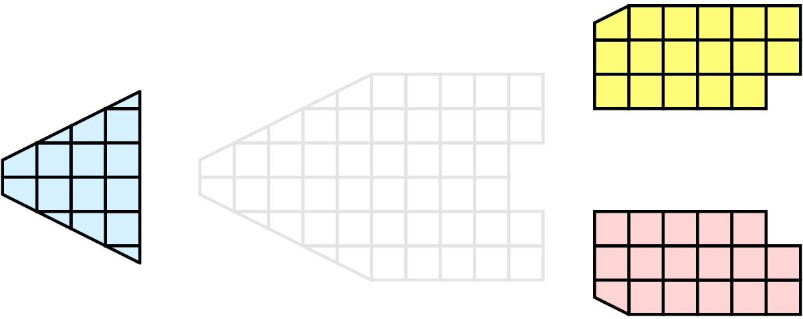
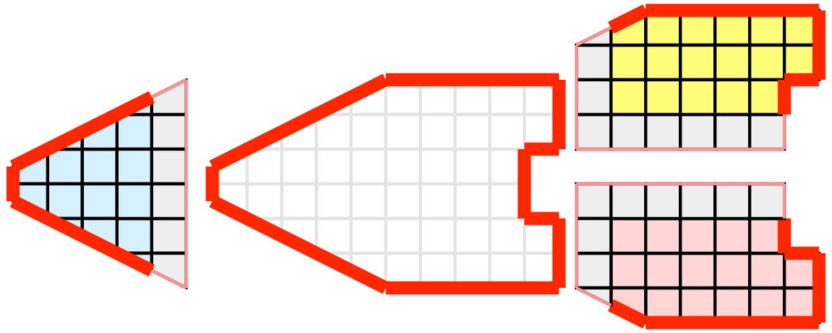
Parallel processing, put simply, implies processing the data in parallel, simultaneously using multiple workers. Typically, these workers are different processes that could be running on a multicore machine or on several nodes of a cluster. Let’s call these ranks. In most data processing and visualization algorithms, work is directly related to the amount of data that needs to be processed, i.e., the number of cells or points in the dataset. Thus, a straight-forward way of distributing the work among ranks is to split an input dataset into multiple chunks and then have each rank operate only an independent set of chunks. Conveniently, for most algorithms, the result obtained by splitting the dataset and processing it separately is same as the result that we’d get if we processed the dataset in a single chunk. There are, of course, exceptions. Let’s try to understand this better with an example. For demonstration purposes, consider this very simplified mesh.

Now, let us say we want to perform visualizations on this mesh using three processes. We can divide the cells of the mesh as shown below with the blue, yellow, and pink regions.
Once partitioned, some visualization algorithms will work by simply allowing each process to independently run the algorithm on its local collection of cells. Take clipping as an example. Let’s say that we define a clipping plane and give that same plane to each of the processes.
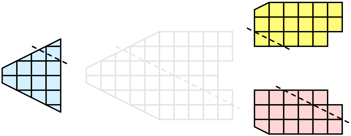
Each process can independently clip its cells with this plane. The end result is the same as if we had done the clipping serially. If we were to bring the cells together (which we would never actually do for large data for obvious reasons), we would see that the clipping operation took place correctly.
8.6.1. Ghost levels
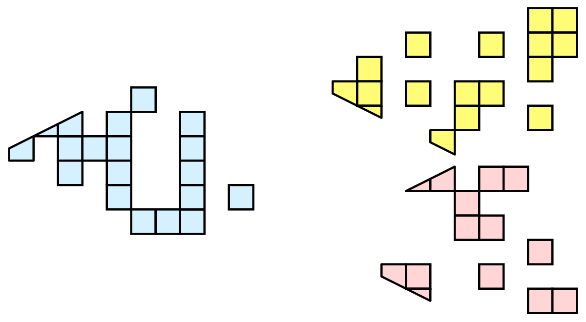
Unfortunately, blindly running visualization algorithms on partitions of cells does not always result in the correct answer. As a simple example, consider the external faces algorithm. The external faces algorithm finds all cell faces that belong to only one cell, thereby, identifying the boundaries of the mesh.
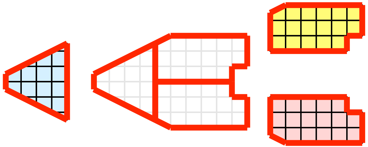
Oops! We see that when all the processes ran the external faces algorithm independently, many internal faces where incorrectly identified as being external. This happens where a cell in one partition has a neighbor in another partition. A process has no access to cells in other partitions, so there is no way of knowing that these neighboring cells exist.
The solution employed by ParaView and other parallel visualization systems is to use ghost cells . Ghost cells are cells that are held in one process but actually belong to another. To use ghost cells, we first have to identify all the neighboring cells in each partition. We then copy these neighboring cells to the partition and mark them as ghost cells, as indicated with the gray colored cells in the following example.
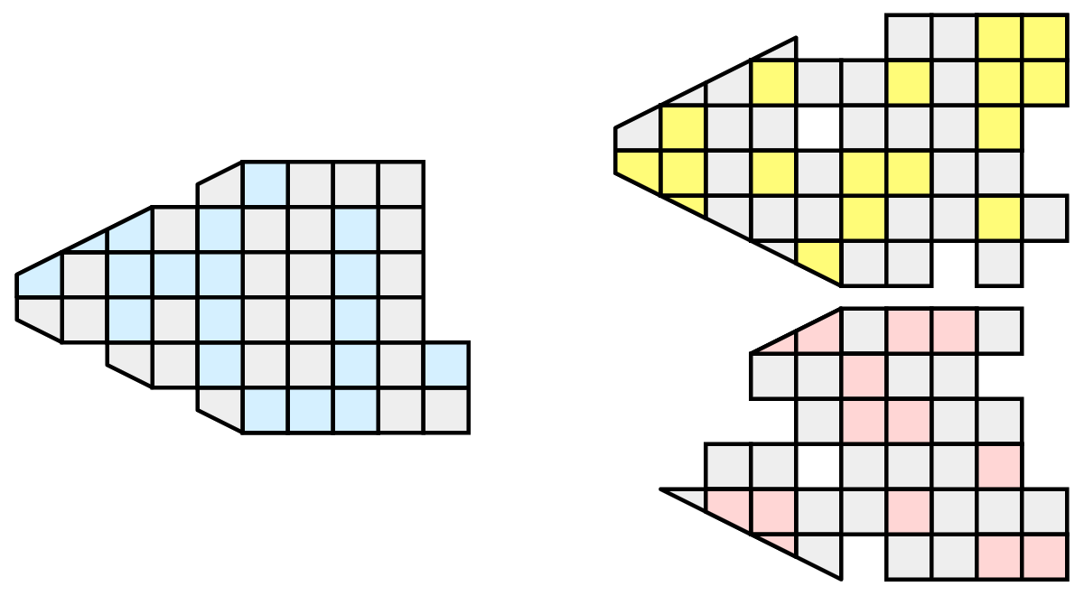
When we run the external faces algorithm with the ghost cells, we see that we are still incorrectly identifying some internal faces as external. However, all of these misclassified faces are on ghost cells, and the faces inherit the ghost status of the cell from which it came. ParaView then strips off the ghost faces, and we are left with the correct answer.
In this example, we have shown one layer of ghost cells: only those cells that are direct neighbors of the partition’s cells. ParaView also has the ability to retrieve multiple layers of ghost cells, where each layer contains the neighbors of the previous layer not already contained in a lower ghost layer or in the original data itself. This is useful when we have cascading filters that each require their own layer of ghost cells. They each request an additional layer of ghost cells from upstream, and then remove a layer from the data before sending it downstream.
8.6.2. Data partitioning
Since we are breaking up and distributing our data, it is prudent to address the ramifications of how we partition the data. The data shown in the previous example has a spatially coherent partitioning. That is, all the cells of each partition are located in a compact region of space. There are other ways to partition data. For example, you could have a random partitioning.
Random partitioning has some nice features. It is easy to create and is friendly to load balancing. However, a serious problem exists with respect to ghost cells.
In this example, we see that a single level of ghost cells nearly replicates the entire dataset on all processes. We have thus removed any advantage we had with parallel processing. Because ghost cells are used so frequently, random partitioning is not used in ParaView.
8.6.3. D3 Filter
The previous section described the importance of load balancing and ghost levels for parallel visualization. This section describes how to achieve that.
Load balancing and ghost cells are handled automatically by ParaView when you are reading structured data (image data, rectilinear grid, and structured grid). The implicit topology makes it easy to break the data into spatially coherent chunks and identify where neighboring cells are located.
It is an entirely different matter when you are reading in unstructured data (poly data and unstructured grid). There is no implicit topology and no neighborhood information available. ParaView is at the mercy of how the data was written to disk. Thus, when you read in unstructured data, there is no guarantee of how well-load balanced your data will be. It is also unlikely that the data will have ghost cells available, which means that the output of some filters may be incorrect.
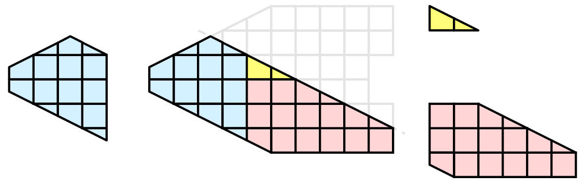
Fortunately, ParaView has a filter that will both balance your unstructured data and create ghost cells. This filter is called D3, which is short for distributed data decomposition. Using D3 is easy; simply attach the filter (located in Filters > Alphabetical > D3) to whatever data you wish to repartition.
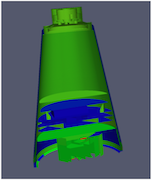
The most common use case for D3 is to attach it directly to your unstructured grid reader. Regardless of how well-load balanced the incoming data might be, it is important to be able to retrieve ghost cell so that subsequent filters will generate the correct data. The example above shows a cutaway of the extract surface filter on an unstructured grid. On the left, we see that there are many faces improperly extracted because we are missing ghost cells. On the right, the problem is fixed by first using the D3 filter.
8.7. Parallel File Readers
Parallel file readers in ParaView are specialized for reading and processing large datasets by dividing file reading across multiple processes simultaneously. These readers typically read portions of file or even separate files concurrently on different processors, significantly reducing the time required to read and parse large datasets compared to sequential reading performed by a single process. Furthermore, when a dataset is read in parallel by distributed multiple processes, it is already divided amongst the processes, which can lead to more efficient subsequent parallel processing steps that fully use the available computing resources. This section includes a comprehensive list of parallel file readers available in ParaView, along with descriptions and usage guidelines.
All the file readers in this section use distributed memory parallelism. Some of these readers also support shared memory parallelism, which is indicated in the description of those readers.
8.7.1. ADIOS2 BP3 File (using Fides), ADIOS2 BP4/5 Directory (using Fides)
paraview.simple.FidesReaderRead ADIOS2 files as image data. Further details about Fides and using it within ParaView can be found at https://fides.readthedocs.io/en/latest/paraview/paraview.html.
8.7.2. AMReX/BoxLib plotfiles (grids)
paraview.simple.AMReXBoxLibGridReaderThis AMReX reader loads data stored in AMReX plt file format. The output of this reader is an overlapping AMR dataset of uniform rectilinear grids.
8.7.3. AMReX/BoxLib plotfiles (particles)
paraview.simple.AMReXBoxLibParticlesReaderReads particle data from AMReX plotfiles.
8.7.4. AMR Velodyne Files
paraview.simple.VelodyneAMRReaderVelodyne is a multi-physics code written by Corvid Technologies. It is a coupled Lagrangian-Eularian code where the Euler equations are solved using AMR. The resulting *.xamr files can be larger than 40GB. This reader was designed to read these files efficiently. The output of this reader is an overlapping AMR dataset.
8.7.5. CGNS Files
paraview.simple.CGNSSeriesReaderThe CGNS reader reads files stored in CGNS format. The default file extension is .cgns. The output of this reader is a multi-block dataset.
This reader handles two types of file series:
temporal file series - where each file is simply a single timestep.
partitioned file series - where each file corresponds to data dumped out from a rank but has all timesteps.
This reader determines the nature of the file series encountered and reads the files accordingly. For partitioned files, the files are distributed among data-processing ranks, while for temporal file series, blocks are distributed among data-processing ranks
8.7.6. CellGrid Files
paraview.simple.CompositeCellGridReaderReader for discontinuous Galerkin and other data in cell-grid format. This reader supports user-extensible cell grid data (for discontinuous fields, novel function spaces, non-isoparametric elements, and other geometric data that does not hold to the assumptions implicit in unstructured grids). If the file contains data in multiple blocks, they are split across ranks in a round-robin fashion. No effort at redistribution is made by the reader.
For more information on how the reader can be extended, see the CellGrid documentation.
8.7.7. Cosmology Files
paraview.simple.CosmoReaderThe Cosmology reader reads a binary file of particle location, velocity, and id creating an unstructured grid. The default file extension is .cosmo64. Reads LANL Cosmo format or Gadget format.
8.7.8. EnSight Gold files (EnSightGoldCombinedReader plugin)
paraview.simple.EnSightGoldCombinedReaderReader for EnSight Gold binary and ASCII files.
Load the EnSightGoldCombinedReader plugin for this reader to be available.
8.7.9. EnSight Gold Server of Server (SOS) files (EnSightSOSGoldReader plugin)
paraview.simple.EnSightSOSGoldReaderReader for EnSight Gold SOS files.
Load the EnSightGoldCombinedReader plugin for this reader to be available.
8.7.10. EnSight Files
paraview.simple.EnSightReaderThe EnSight reader reads files in the format produced by EnSight. EnSight 6 and Gold files (both ASCII and binary) are supported. The default xtension is .case. The output of this reader is a multiblock dataset.
This reader is built-in to ParaView and does not require any plugin to be loaded.
8.7.11. EnSight Master Server Files
paraview.simple.EnSightMasterServerReader8.7.12. ENZO AMR Particles Reader
paraview.simple.ENZOAMRParticlesReaderLoads AMR particle files produced by the Enzo adaptive mesh refinement simulation code: https://enzo-project.org/
8.7.13. Exodus II (legacy)
paraview.simple.LegacyExodusIIReaderLoad the LegacyExodusIIReader plugin for this reader to be available. For comprehensive information about Exodus II file conventions and how they are treated in ParaView, please see the section Exodus.
8.7.14. Metafile for restarted exodus outputs
paraview.simple.LegacyRestartedSimExodusReaderLoad the LegacyExodusIIReader plugin for this reader to be available.
8.7.15. Fides Data Model File (JSON)
paraview.simple.FidesJSONReaderReads an ADIOS2 file using the Fides library. For more information on the JSON model schema, please see https://fides.readthedocs.io/en/latest/schema/schema.html.
8.7.16. GenericIO files to UnstructuredGrid
paraview.simple.GenericIOReaderReads a cosmology file into an unstructured grid.
8.7.17. GenericIO files to MultiBlockDataSet
paraview.simple.GenericIOMultiBlockReaderReads a cosmology file into a multiblock dataset
8.7.18. IOSS Files (Exodus II and CGNS)
paraview.simple.IOSSReaderReads Exodus II and CGNS files using the IOSS library. The reader produces unstructured grids when reading Exodus II files and structured grids when reading CGNS files. For comprehensive information about Exodus II file conventions and how they are treated in ParaView, please see the section Exodus.
8.7.19. IOSS Files (exdg)
paraview.simple.IOSSCellGridReaderReads CellGrid datasets from Exodus II files using the IOSS library. Currently, continuous Galerkin (CG) fields are not supported; only discontinuous Galerkin (DG) fields will be read until a convention is created for storing shared degrees of freedom.
8.7.20. LSDyna
paraview.simple.LSDynaReaderThis reader reads LS-Dyna databases (d3plot files).
8.7.21. Nek5000 Files
paraview.simple.Nek5000ReaderReads Nek5000 data files, producing an unstructured grid dataset.
8.7.22. Nrrd Raw Image Files
paraview.simple.NrrdReaderNrrd reader reads raw image data much like the Raw Image Reader except that it will also read metadata information in the Nrrd format. This means that the reader will automatically set information like file dimensions. There are several limitations on what type of nrrd files we can read. This reader only supports nrrd files in raw format. Other encodings like ASCII and hex will result in errors. When reading in detached headers, this only supports reading one File that is detached.
8.7.23. OpenFOAM Files
paraview.simple.OpenFOAMReaderReads OpenFOAM data files, producing multiblock datasets. File requests are multithreaded to hide latency on network file systems.
8.7.24. PIO Dump Files
paraview.simple.PIOReaderPIO is a file format in support of xRage, a physics code from Los Alamos National Laboratory. The input file (.pio) opened by the PIO reader is an ASCII description of the data files within a dump directory numbered by cycle. The reader uses a PIOData class to read the file and a PIOAdaptor to build an unstructured or hypertree grid from the data. Requested data is filled into the structures.
8.7.25. PLOT3D Meta Files
paraview.simple.PLOT3DMetaFileReaderReads a metadata file that describes the geometry and solution files of a PLOT3D dataset.
8.7.26. PLOT3D Solution Files
paraview.simple.PLOT3DReaderThe PLOT3D reader can read both ASCII and binary PLOT3D files. The default file extension for the geometry files is .xyz, and the default file extension for the solution files is .q. The output of this reader is a multiblock dataset containing curvilinear (structured grid) datasets.
8.7.27. POP Ocean NetCDF (Rectilinear)
paraview.simple.ParallelNetCDFPOPreaderReads HDF5 files generated from xRage, a physics code from Los Alamos National Laboratory. The data is first read in by one process, then it is partitioned and distributed to all other processes.
8.7.28. POP Ocean NetCDF (Unstructured)
paraview.simple.UnstructuredNetCDFPOPreaderThe reader reads regular rectilinear grid (image/volume) data from a NetCDF file and turns it into an unstructured spherical grid.
8.7.29. Rage HDF Files
paraview.simple.HDF5RageReaderReads HDF dump files generated from xRage, a LANL physics code, using the PIO (Parallel Input Output) library.
8.7.30. SLAC Mesh Files
paraview.simple.SLACDataReaderA reader for a data format used by Omega3p, Tau3p, and several other tools used at the Standford Linear Accelerator Center (SLAC). The underlying format uses NetCDF to store arrays, but also imposes several conventions to form an unstructured grid of elements.
8.7.31. SpyPlot CTH dataset
paraview.simple.SpyPlotReaderThe Spy Plot reader loads an ASCII meta-file called the “case” file (extension .spcth). The case file lists all the binary files containing the dataset. This reader produces hierarchical datasets.
8.7.32. Case file for restarted CTH outputs
paraview.simple.RestartedSimSpyPlotReaderReads a metadata file listing restart files from multiple restarts of the CTH simulation code and treats them as one continuous dataset. For additional details on restarted SPCTH files, see the section SPCTH.
8.7.33. VPIC Files
paraview.simple.VPICReaderVPIC is a 3D kinetic plasma particle-in-cell simulation. The input file (.vpc) opened by the VPIC reader is an ASCII description of the data files which are written one file per processor, per category and per time step. These are arranged in subdirectories per category (field data and hydrology data) and then in time step subdirectories. This is a distributed reader.
8.7.34. Legacy VTK Files (partitioned)
paraview.simple.PartitionedLegacyVTKReaderThe Partitioned Legacy VTK reader loads files stored in VTK’s partitioned legacy file format (before VTK 4.2, although still supported). The expected file extension is .pvtk. The type of the dataset may be structured grid, uniform rectilinear grid (image/volume), non-uniform rectilinear grid, unstructured grid, or polygonal.
Details about the legacy VTK file format can be found at https://docs.vtk.org/en/latest/vtk_file_formats/vtk_legacy_file_format.html
8.7.35. VTKHDF Files
paraview.simple.VTKHDFReaderReads VTKHDF serial or parallel data files. All data types are read from the same reader. This reader also supports file series.
For comprehensive details about the VTKHDF file format, please see https://docs.vtk.org/en/latest/vtk_file_formats/vtkhdf_file_format/
8.7.36. VTK ImageData Files (partitioned)
paraview.simple.XMLPartitionedImageDataReaderThe XML Partitioned Image Data reader reads the partitioned VTK image data file format. It reads the partitioned format’s summary file and then the associated VTK XML image data files. This reader also supports file series.
Details about the legacy VTK file format can be found at https://docs.vtk.org/en/latest/vtk_file_formats/vtk_legacy_file_format.html
8.7.37. (VTK) HyperTreeGrid (partitioned)
paraview.simple.XMLPartitionedHyperTreeGridReaderThe XML Partitioned Hyper Tree Grid reader reads the partitioned VTK htg data file format. It reads the partitioned format’s summary file and then the associated VTK XML htg data files. This reader also supports file series.
Details about the legacy VTK file format can be found at https://docs.vtk.org/en/latest/vtk_file_formats/vtk_legacy_file_format.html
8.7.38. VTK PolyData Files (partitioned)
paraview.simple.XMLPartitionedPolyDataReaderThe XML Partitioned Polydata reader reads the partitioned VTK polydata file format. It reads the partitioned format’s summary file and then the associated VTK XML polydata files. This reader also supports file series.
Details about the legacy VTK file format can be found at https://docs.vtk.org/en/latest/vtk_file_formats/vtk_legacy_file_format.html
8.7.39. VTK RectilinearGrid Files (partitioned)
paraview.simple.XMLPartitionedRectilinearGridReaderThe XML Partitioned Rectilinear Grid reader reads the partitioned VTK rectilinear grid file format. It reads the partitioned format’s summary file and then the associated VTK XML rectilinear grid files. This reader also supports file series.
Details about the legacy VTK file format can be found at https://docs.vtk.org/en/latest/vtk_file_formats/vtk_legacy_file_format.html
8.7.40. VTK StructuredGrid Files (partitioned)
paraview.simple.XMLPartitionedStructuredGridReaderThe XML Partitioned Structured Grid reader reads the partitioned VTK structured grid data file format. It reads the partitioned format’s summary file and then thed associated VTK XML structured grid data files. This reader also supports file series.
Details about the legacy VTK file format can be found at https://docs.vtk.org/en/latest/vtk_file_formats/vtk_legacy_file_format.html
8.7.41. VTK Table (partitioned)
paraview.simple.XMLPartitionedTableReaderThe XML Partitioned Table reader reads the partitioned VTK table data file format. It reads the partitioned format’s summary file and then the associated VTK XML table data files.
Details about the legacy VTK file format can be found at https://docs.vtk.org/en/latest/vtk_file_formats/vtk_legacy_file_format.html
8.7.42. VTK UnstructuredGrid Files (partitioned)
paraview.simple.XMLPartitionedUnstructuredGridReaderThe XML Partitioned Unstructured Grid reader reads the partitioned VTK unstructured grid data file format. It reads the partitioned format’s summary file and then the associated VTK XML unstructured grid data files. This reader also supports file series.
Details about the legacy VTK file format can be found at https://docs.vtk.org/en/latest/vtk_file_formats/vtk_legacy_file_format.html
8.7.43. VTX reader: ADIOS2 BP3 File, VTX reader: ADIOS2 BP4 Directory
paraview.simple.ADIOS2VTXReaderReads an ADIOS2 BP file with embedded VTK XML Schema for vti (Image) and vtu (UnstructuredGrid) types either as an attribute or as a subfile.
8.7.44. WindBlade Data
paraview.simple.WindBladereaderWindBlade/Firetec is a simulation dealing with the effects of wind on wind turbines or on the sread of fires. It produces three outputs - a StructuredGrid for the wind data fields, a StructuredGrid for the ground topology, and a PolyData for turning turbine blades. The input file (.wind) opened by the WindBlade reader is an ASCII description of the data files expected. Data is accumulated by the simulation processor and is written one file per time step. WindBlade can deal with topology if a flag is turned on and expects (x,y) data for the ground. It also can deal with turning wind turbines from other time step data files which gives polygon positions of segments of the blades and data for each segment.
8.7.45. Xdmf Reader (XDMF 2)
paraview.simple.XDMFReaderThe XDMF reader reads files in XDMF 2 format. The expected file extension is .xmf. Metadata is stored in the XDMF file using an XML format, and large attribute arrays are stored in a corresponding HDF5 file. The output may be unstructured grid, structured grid, or rectiliner grid. See http://www.xdmf.org for a description of the file format.
8.7.46. Xdmf3 Reader
paraview.simple.Xdmf3ReaderTThe output data produced by this reader depends on the number of grids in the data file. If the data file has a single domain with a single grid, then the output type is a dataset of the appropriate type, otherwise it’s a multiblock data set. This reader treats a file series as a time series rather than as a spatial partition.
8.7.47. Xdmf3 Reader (Top Level Partition)
paraview.simple.Xdmf3ReaderSThe output data produced by this reader depends on the number of grids in the data file. If the data file has a single domain with a single grid, then the output type is a dataset of the appropriate type, otherwise it’s a multiblock data set. Treats a file series as a spatial partition rather than as a time series.
8.8. Parallel File Writers
ParaView can save files to various parallel file formats. The following is a comprehensive list of parallel file writers available in ParaView, along with their descriptions and usage guidelines. Unless otherwise noted, parallel writers typically save the portions of datasets that are local to each process in separate data files and produce a summary file that references the individual data files.
8.8.1. ADIOS2 BP File
paraview.simple.FidesWriterWrite ADIOS2 files using Fides. Further details about Fides and using it within ParaView can be found at https://fides.readthedocs.io/en/latest/paraview/paraview.html.
8.8.2. CGNS Files
paraview.simple.CGNSWriterThe CGNS writer writes files stored in CGNS format. The file extension is .cgns. This writer can write structured grids, poly data, unstructured grids or a multi-block dataset containing these data types.
8.8.3. Comma or Tab Delimited Files
paraview.simple.CSVWriterWriter to write comma- or tab-delimited files from any dataset. The output is a single file containing the data from all ranks.
8.8.4. EnSight File
paraview.simple.EnSightWriterWriter to write unstructured grid data as an EnSight file. Binary files written on one system may not be readable on other systems. Be sure to specify the endian-ness of the file when reading it into EnSight.
8.8.5. Generic IO Files
paraview.simple.GenericIOWriterWriter to write GenericIO files from multiblock data, each block becomes one rank’s data in the written GenericIO file.
8.8.6. Houdini File Format
paraview.simple.HoudiniWriterWriter to write polygonal data in ASCII Houdini .geo (pre-v12.0) format. This writer gathers all the geometry to the root node and saves one file.
8.8.7. IOSS Exodus File
paraview.simple.IOSSWriterWrite Exodus II files using the IOSS libraries. This writer expects datasets to have a structure that matches the datasets read by the IOSS Exodus File reader. In addition, if global point or cell Ids are missing from the dataset, this writer will generate them. It will also make a best-effort attempt to generate element sides.
8.8.8. ExodusII File (legacy)
paraview.simple.LegacyExodusIIWriterLegacy writer to write Exodus II files. Available through the LegacyExodusWriter plugin.
8.8.9. Wavefront OBJ File Format
paraview.simple.POBJWriterThis writer gathers polydata from all ranks and writes it to a single file in the Wavefront OBJ format. Written files contain the geometry including lines, triangles and polygons. Normals and texture coordinates on points are also written if they exist.
8.8.10. OpenVDB File Format
paraview.simple.OpenVDBWriterWrites image data or point sets to OpenVDB files. A separate grid is written for each rank.
8.8.11. Legacy VTK Files (polydata)
paraview.simple.PDataSetWriterPolyDataWriter to save polydata in VTK’s legacy file format. This writer gathers all the geometry to the root node and saves one file.
Details about the legacy VTK file format can be found at https://docs.vtk.org/en/latest/vtk_file_formats/vtk_legacy_file_format.html
8.8.12. Legacy VTK Files (unstructured grid)
paraview.simple.PDataSetWriterUnstructuredGridWriter to save unstructured grids in VTK’s legacy file format. This writer gathers all the geometry to the root node and saves one file.
Details about the legacy VTK file format can be found at https://docs.vtk.org/en/latest/vtk_file_formats/vtk_legacy_file_format.html
8.8.13. PVTK Hyper Tree Grid Files (XML)
paraview.simple.XMLPHyperTreeGridWriterWriter to write hyper tree grid in a XML-based VTK data file. Can be used for parallel writing.
8.8.14. PVTK ImageData Files (XML)
paraview.simple.XMLPImageDataWriterWriter to write image data in a XML-based VTK data file.
Details about the legacy VTK file format can be found at https://docs.vtk.org/en/latest/vtk_file_formats/vtkxml_file_format.html
8.8.15. VTK Multi Block Files (XML)
paraview.simple.XMLMultiBlockDataWriterWriter to write a multiblock dataset in a XML-based VTK data file. When used for parallel writing, each rank saves data for one or more blocks, and the root node saves a summary file that references the individual block files.
Details about the legacy VTK file format can be found at https://docs.vtk.org/en/latest/vtk_file_formats/vtkxml_file_format.html
8.8.16. VTK Multi Block Files (hypertree grid)
paraview.simple.SerialHTGMultiBlockWrites hypertree grids to multiblock files. The same as the writer for PVTK XML MultiBlockDataSet Files, but specialized to hypertree grids.
Details about the legacy VTK file format can be found at https://docs.vtk.org/en/latest/vtk_file_formats/vtkxml_file_format.html
8.8.17. VTK Partitioned Data Set Files (XML)
paraview.simple.XMLPPartitionedDataSetWriterWriter to write a partitioned dataset in a XML-based VTK data file. When used for parallel writing, each rank saves data for one or more partitions, and the root node saves a summary file that references the individual partition files.
Details about the legacy VTK file format can be found at https://docs.vtk.org/en/latest/vtk_file_formats/vtkxml_file_format.html
8.8.18. VTK PartitionedDataSetCollection Files (XML)
paraview.simple.XMLPartitionedDataSetCollectionWriterWriter to write a partitioned dataset collection in a XML-based VTK data file. When used for parallel writing, each rank saves data for one or more partitions, and the root node saves a summary file that references the individual partitioned datasets in the collection.
Details about the legacy VTK file format can be found at https://docs.vtk.org/en/latest/vtk_file_formats/vtkxml_file_format.html
8.8.19. PVTK PolyData Files (XML)
paraview.simple.XMLPPolyDataWriterWriter to write polydata in a XML-based VTK data file. Can be used for parallel writing.
Details about the legacy VTK file format can be found at https://docs.vtk.org/en/latest/vtk_file_formats/vtkxml_file_format.html
8.8.20. PVTK RectilinearGrid Files (XML)
paraview.simple.XMLPRectilinearGridWriterWriter to write rectilinear grid in a XML-based VTK data file. Can be used for parallel writing.
Details about the legacy VTK file format can be found at https://docs.vtk.org/en/latest/vtk_file_formats/vtkxml_file_format.html
8.8.21. PVTK StructuredGrid Files (XML)
paraview.simple.XMLPStructuredGridWriterWriter to write structured grid in a XML-based VTK data file. Can be used for parallel writing.
Details about the legacy VTK file format can be found at https://docs.vtk.org/en/latest/vtk_file_formats/vtkxml_file_format.html
8.8.22. VTK AMR Files (XML)
paraview.simple.XMLUniformGridAMRWriterWriter to write an AMR data-set (overlapping/non-overlapping) in a XML-based VTK data file.
Details about the legacy VTK file format can be found at https://docs.vtk.org/en/latest/vtk_file_formats/vtkxml_file_format.html
8.8.23. Stereo Lithography File Format
paraview.simple.PSTLWriterWrites stereo lithography (.stl) files in either ASCII or binary form. This writer gathers all the geometry to the root node and saves one file.
8.8.24. VTKHDF Files
paraview.simple.VTKHDFWriterThe VTKHDF Writer writes files in VTKHDF format, using extension .vtkhdf, a format derived from HDF5. Currently, it supports writing Unstructured Grid and PolyData datasets, possibly transient, as well as composite types Partitioned Dataset Collection and Multiblock Dataset, without transient support.
Details about the VTKHDF file format can be found at https://docs.vtk.org/en/latest/vtk_file_formats/vtkhdf_file_format/
8.8.25. Xdmf3 Data File
paraview.simple.Xdmf3WriterThe Xdmf3 writer writes VTK data objects to XDMF format and and when run in parallel under MPI each rank writes only the data it is responsible for.
8.9. Ghost Cells Generation
If your unstructured grid data is already partitioned satisfactorily but does
not have ghost cells, it is possible to generate them using the Ghost Cells
filter. This filter can be attached to a source just like the D3 filter.
Unlike D3 , it will not repartition the dataset, it will only generate
ghost cells, which is needed for some algorithms to execute correctly.
The Ghost Cells filter has several options. Build If Required
tells the filter to generate ghost cells only if required by a downstream filter.
Since computing ghost cells is a computationally and communications intensive
process, turning this option on can potentially save a lot of processing time.
The Minimum Number Of Ghost Levels specifies at least how many ghost levels
should be generated if Build If Required is off. Downstream filters may request
more ghost levels than this minimum, in which case the Ghost Cells
will generate the requested number of ghost levels. The Use Global Ids option
makes use of a GlobalIds array if it is present if on. If off, ghost cells are
determined by coincident points.
8.10. ParaView architecture
Before we see how to use ParaView for parallel data processing, let’s take a closer look at the ParaView architecture. ParaView is designed as a three-tier client-server architecture. The three logical units of ParaView are as follows.
Data Server The unit responsible for data reading, filtering, and writing. All of the pipeline objects seen in the pipeline browser are contained in the data server. The data server can be parallel.
Render Server The unit responsible for rendering. The render server can also be parallel, in which case built-in parallel rendering is also enabled.
Client The unit responsible for establishing visualization. The client controls the object creation, execution, and destruction in the servers, but does not contain any of the data (thus allowing the servers to scale without bottlenecking on the client). If there is a GUI, that is also in the client. The client is always a serial application.
These logical units need not by physically separated. Logical units are often embedded in the same application, removing the need for any communication between them. There are three modes in which you can run ParaView.
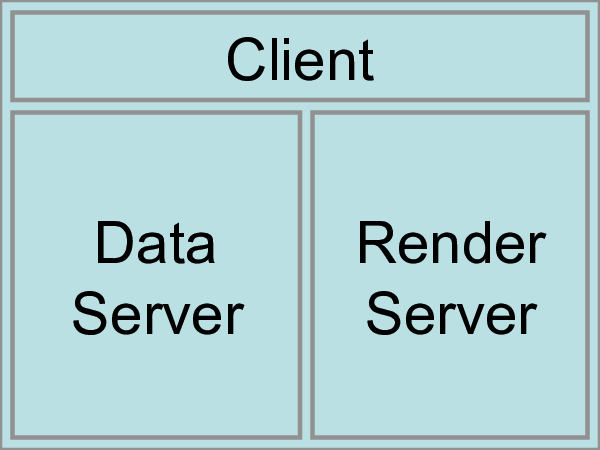
The first mode, with which you are already familiar, is
standalone mode. In standalone mode, the client, data server,
and render server are all combined into a single serial application. When
you run the paraview application, you are automatically connected
to a builtin server so that you are ready to use the full
features of ParaView.
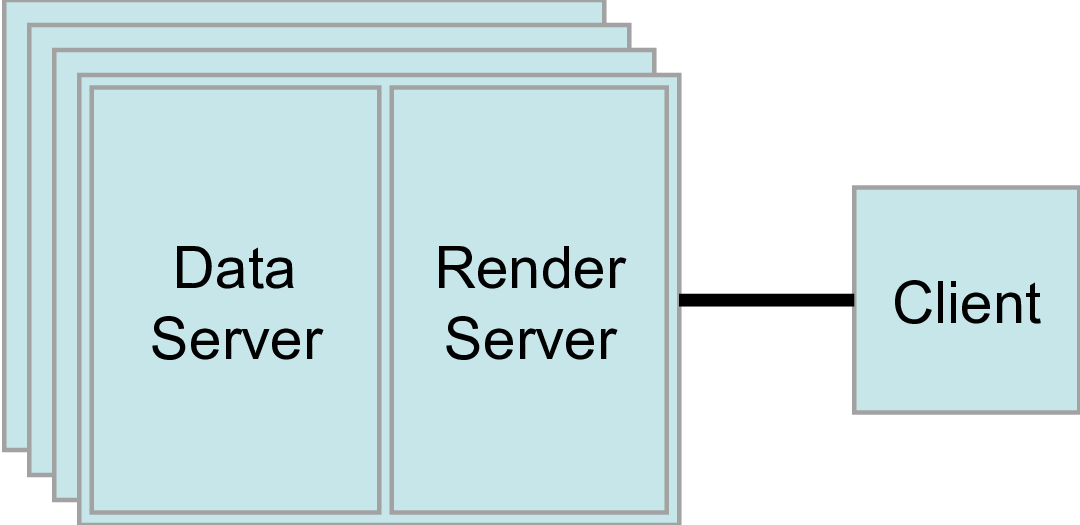
The second mode is client-server mode. In client-server mode,
you execute the pvserver program on a parallel machine and
connect to it with the paraview client application (or pvpython). The
pvserver program has both the data server and render server
embedded in it, so both data processing and rendering take place there.
The client and server are connected via a socket, which is assumed to be a
relatively slow mode of communication, so data transfer over this socket is
minimized. We saw this mode of operation in
Section 8.2.
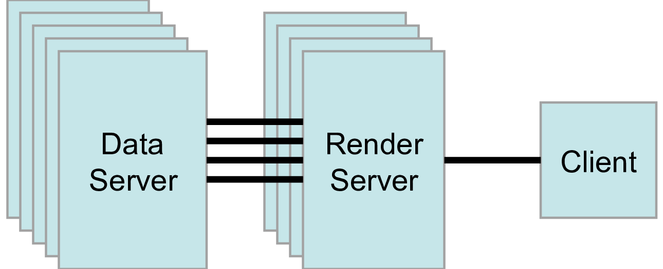
The third mode is client-render server-data server mode. In this mode, all three logical units are running in separate programs. As before, the client is connected to the render server via a single socket connection. The render server and data server are connected by many socket connections, one for each process in the render server. Data transfer over the sockets is minimized.
Although the client-render server-data server mode is supported, we almost
never recommend using it. The original intention of this mode is to take
advantage of heterogeneous environments where one might have a large,
powerful computational platform and a second smaller parallel machine with
graphics hardware in it. However, in practice, we find any benefit is
almost always outstripped by the time it takes to move geometry from the
data server to the render server. If the computational platform is much
bigger than the graphics cluster, then use software rendering on the large
computational platform. If the two platforms are about the same size, just
perform all the computation on the graphics cluster. The executables used for
this mode are paraview (or pvpython) (acting as the client), pvdataserver for
the data-server, and pvrenderserver for the render-server.
8.11. Parallel processing in paraview and pvpython
To leverage parallel processing capabilities in paraview or pvpython, one has
to use remote visualization, i.e., one has to connect to a pvserver. The
processing for connecting to this pvserver is not different from what we
say in Section 8.2
and Section 8.3. The only thing that changes is how the
pvserver is launched.
You can start pvserver to run on more than one processing core
using mpirun
.
mpirun -np 4 pvserver
This will run pvserver on four processing cores. It will still listen
for an incoming connection from a client on the default port. The big
difference when running pvserver this way is that when data is loaded
from a source, it will be distributed across the four cores if the
data source is parallel aware and supports distributing the data
across the different processing cores.
To see how this data is distributed, run pvserver as the command above and
connect to it with paraview. Next, create another Sphere source
using Source > Sphere. Change the array to color by to
vtkProcessId . You will see an image like Figure Fig. 8.16.
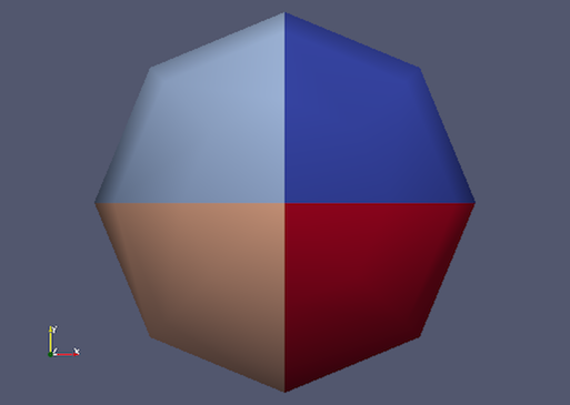
Fig. 8.16 Sphere source colored by vtkProcessId array that encodes
the processing core on which the sphere data resides. Here, the sphere
data is split among the four processing cores invoked by the
command mpirun -np 4 pvserver.
If a data reader or source is not parallel aware, you can still get
the benefits of spreading the data among processing cores by using the
D3 filter. This filter partitions a dataset into convex regions
and transfers each region to a different processing core. To see an
example of how D3 partitions a dataset, create a Source > Wavelet
while paraview is still connected to the pvserver. Next, select
Filters > Alphabetical > D3 and click Apply . The output of D3
will not initially appear different from the original wavelet source.
If you color by vtkProcessId , however, you will see the four
partitions that have been distributed to the server processing cores.
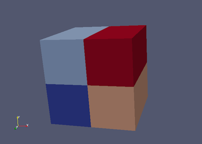
Fig. 8.17 Wavelet source processed by the D3 filter and colored by vtkProcessId
array. Note how four regions of the image data are split evenly among the four
processing cores when pvserver is run with mpirun -np 4 pvserver .
8.12. Using pvbatch
In Section 8.11, we said that to use parallel
processing capabilities, one has to use remote visualization, i.e., one must use
ParaView in a client-server mode with the client (paraview or pvpython)
connecting to a server (pvserver) that is being run in parallel using
mpirun
. However, there is one exception: pvbatch. pvpython and
pvbatch are quite similar in that both are similarly to the python
executable that can be used to run Python scripts. The extra thing that these
executables do when compared with the standard python is that they
initialize the environment so that any scripts that you run will be able to
locate the ParaView Python modules and libraries automatically. pvpython is
exactly like the paraview executable without the GUI. You can think of it as
the GUI from paraview is replaced by a Python interpreter in pvpython.
pvbatch, on the other hand, can be thought of a pvserver where, instead of
taking the control command from a remote client (paraview or pvpython), in
pvbatch, the commands are taken from a Python script that is executed in the
pvbatch executable itself. Since pvbatch is akin to the pvserver, unlike
pvpython, it can be run in parallel using mpirun
. In that case,
the root rank (or the first rank or the rank with index $0$) is the one that
acts as the client, interpreting the Python script to execute the commands.
Since pvbatch is designed to act is its own server, you cannot connect to a
remote server in the Python script, i.e., you cannot use simple.Connect .
Furthermore, pvbatch is designed for batch operation, which means that you can only
specify the Python script as a command line argument. Unlike pvpython, you
cannot run this executable to get an interactive shell to enter Python commands.
# process the sample.py script in single process mode.
> pvbatch sample.py

# process the sample.py script in parallel.
> mpirun -np 4 pvbatch sample.py
In general, you should use pvpython if you will be using the interpreter
interactively and pvbatch if you are running in parallel.
8.13. Fetching data to the client
Section 4.3 describes how to obtain information
about a data object, but not how to access the data object itself. This
section describes several ways to access data from within a Python script. The
client/server nature of ParaView requires a couple steps to access the raw data.
The Python script runs on the client side in either pvpython or paraview, so
one step involves moving the data from the server to the client. This can be
accomplished with the following:
from paraview.simple import *
Connect("myhost")

# Create a sphere source on myhost
s = Sphere()
full_sphere = servermanager.Fetch(s)
Here, the full dataset is moved from the server to the client.
The second step is required to deal with the fact that data on the remote server
may be split across distributed processes. By default,
servermanager.Fetch(s) appends all the pieces on the different remote
processes and produces the appended dataset on the client. The exact
append operation depends on the type of dataset being retrieved. Composite datasets
are merged by treating the dataset piece on each distributed process as a block
merged into a new multiblock dataset, polygonal datasets are appended into a single
polygonal dataset, rectilinear grids are appended into a single rectilinear grid,
and other datasets are appended into an unstructured grid. Distributed image
datasets cannot currently be fetched to the client. Care must be taken when
fetching an entire dataset to the client because the data that fits on many
distributed processes on a remote system may not fit in client memory.
Another option is to fetch just a single piece of the dataset on one remote
process to the client. To do this, pass the rank number of the remote process from
which you want to retrieve the data to the Fetch function, e.g.,
# Retrieve the piece of the dataset on remote process 2
s = Sphere()
sphere_piece = servermanager.Fetch(s, 2)
Lastly, servermanager.Fetch provides a way to apply helper filters to the
dataset that run at two stages. The filter for the first stage is applied to the
data on each remote process, and the filter for the second stage is applied to the
results from the first stage after they are gathered to the root server process.
The results from the second stage of filtering are then transferred from the root
server process to the client.
In the next example, the Extract Surface filter is applied to a source with
data on each process in the first stage. The results are then assembled with the
Append Geometry filter and sent to the client.
s = Sphere()
extract = servermanager.filters.ExtractSurface()
append = servermanager.filters.AppendGeometry()
full_surface = servermanager.Fetch(s, extract, append)
The second filter must be able to accept multiple connections and handle the output dataset type from the first filter.
8.14. Rendering
Rendering is the process of synthesizing the images that you see based on your data. The ability to effectively interact with your data depends highly on the speed of the rendering. Thanks to advances in 3D hardware acceleration, fueled by the computer gaming market, we have the ability to render 3D quickly even on moderately-priced computers. But, of course, the speed of rendering is proportional to the amount of data being rendered. As data gets bigger, the rendering process naturally gets slower.
To ensure that your visualization session remains interactive, ParaView supports two modes of rendering that are automatically flipped as necessary. In the first mode, still render , the data is rendered at the highest level of detail. This rendering mode ensures that all of the data is represented accurately. In the second mode, interactive render , speed takes precedence over accuracy. This rendering mode endeavors to provide a quick rendering rate regardless of data size.
While you are interacting with a 3D view (for example, rotating, panning, or zooming with the mouse), ParaView uses an interactive render. This is because, during the interaction, a high frame rate is necessary to make these features usable and because each frame is immediately replaced with a new rendering while the interaction is occurring so that fine details are less important during this mode. At any time when interaction of the 3D view is not taking place, ParaView uses a still render so that the full detail of the data is available as you study it. As you drag your mouse in a 3D view to move the data, you may see an approximate rendering. The full detail will be presented as soon as you release the mouse button.
The interactive render is a compromise between speed and accuracy. As such, many of the rendering parameters concern when and how lower levels of detail are used.
8.14.1. Basic Rendering Settings
Some of the most important rendering options are the LOD parameters. During interactive rendering, the geometry may be replaced with a lower level of detail ( LOD ), an approximate geometry with fewer polygons.
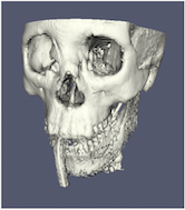
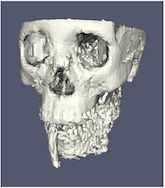
The resolution of the geometric approximation can be controlled. In the proceeding images, the left image is the full resolution, the middle image is the default decimation for interactive rendering, and the right image is ParaView’s maximum decimation setting.
The 3D rendering parameters are located in the settings dialog box, which is
accessed in the menu from the Edit > Settings menu
(ParaView > Preferences on the Mac). The rendering options in the dialog
are in the Render View tab.
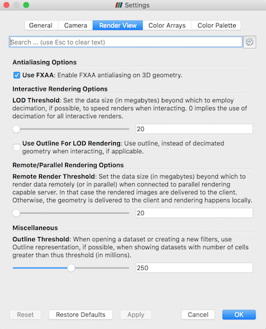
The options pertaining to the geometric decimation for interactive
rendering are located in a section labeled Interactive Rendering Options .
Some of these options are considered advanced, so to access
them, you have to either toggle on the advanced options with the
 button or search for the option using the edit box at
the top of the dialog. The interactive rendering options include the
following.
button or search for the option using the edit box at
the top of the dialog. The interactive rendering options include the
following.
LOD Threshold: Set the data size at which to use a decimated geometry in interactive rendering. If the geometry size is under this threshold, ParaView always renders the full geometry. Increase this value if you have a decent graphics card that can handle larger data. Try decreasing this value if your interactive renders are too slow.LOD Resolution: Set the factor that controls how large the decimated geometry should be. This control is set to a value between 0 and 1. 0 produces a very small number of triangles but, possibly, with a lot of distortion. 1 produces more detailed surfaces but with larger geometry.Non Interactive Render Delay: Add a delay between an interactive render and a still render. ParaView usually performs a still render immediately after an interactive motion is finished (for example, releasing the mouse button after a rotation). This option can add a delay that can give you time to start a second interaction before the still render starts, which is helpful if the still render takes a long time to complete.Use Outline For LOD Rendering: Use an outline in place of decimated geometry. The outline is an alternative for when the geometry decimation takes too long or still produces too much geometry. However, it is more difficult to interact with just an outline.
ParaView contains many more rendering settings. Here is a summary of some other settings that can effect the rendering performance regardless of whether ParaView is run in client-server mode or not. These options are spread among several categories, and several are considered advanced.
Translucent Rendering OptionsDepth Peeling: Enable or disable depth peeling. Depth peeling is a technique ParaView uses to properly render translucent surfaces. With it, the top surface is rendered and then “peeled away” so that the next lower surface can be rendered and so on. If you find that making surfaces transparent really slows things down or renders completely incorrectly, then your graphics hardware may not be implementing the depth peeling extensions well; try shutting off depth peeling.Depth Peeling for Volumes: Include volumes in depth peeling to correctly intermix volumes and translucent polygons.Maximum Number Of Peels: Set the maximum number of peels to use with depth peeling. Using more peels allows more depth complexity, but allowing less peels runs faster. You can try adjusting this parameter if translucent geometry renders too slow or translucent images do not look correct.
MiscellaneousOutline Threshold: When creating very large datasets, default to the outline representation. Surface representations usually require ParaView to extract geometry of the surface, which takes time and memory. For data with sizes above this threshold, use the outline representation, which has very little overhead, by default instead.Show Annotation: Show or hide annotation providing rendering performance information. This information is handy when diagnosing performance problems.
Note that this is not a complete list of ParaView rendering settings. We have left out settings that do not significantly affect rendering performance. We have also left out settings that are only valid for parallel client-server rendering, which are discussed in Section 8.14.4.
8.14.2. Basic Parallel Rendering
When performing parallel visualization, we are careful to ensure that the data remains partitioned among all of the processes up to and including the rendering processes. ParaView uses a parallel rendering library called IceT . IceT uses a sort-last algorithm for parallel rendering. This parallel rendering algorithm has each process independently render its partition of the geometry and then composites the partial images together to form the final image.
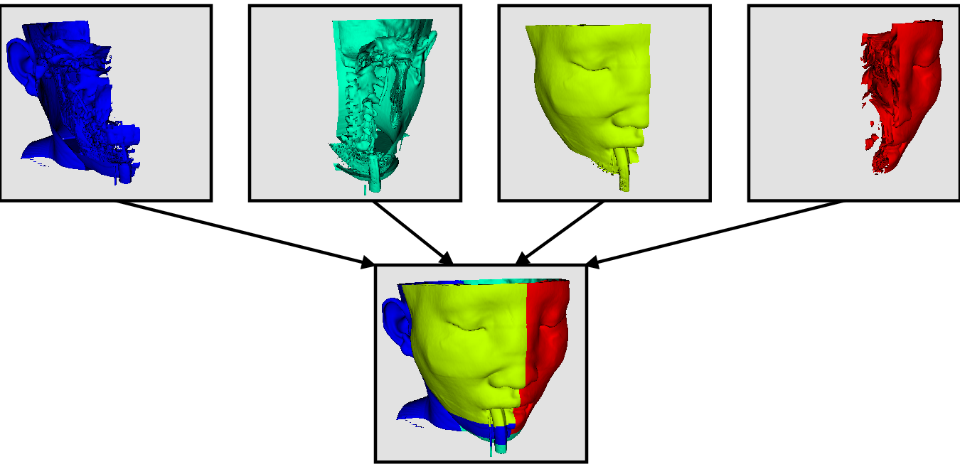
The preceding diagram is an oversimplification. IceT contains multiple parallel image compositing algorithms such as binary tree , binary swap , and radix-k that efficiently divide work among processes using multiple phases.
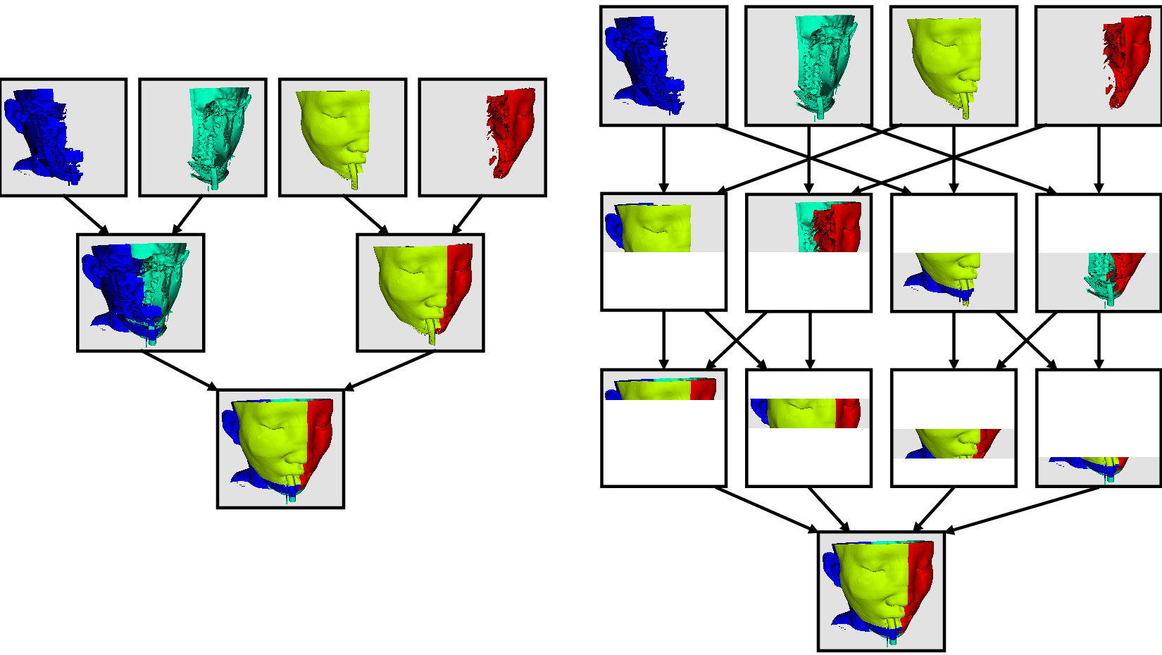
The wonderful thing about sort-last parallel rendering is that its efficiency is completely insensitive to the amount of data being rendered. This makes it a very scalable algorithm and well suited to large data. However, the parallel rendering overhead does increase linearly with the number of pixels in the image. Consequently, some of the rendering parameters deal with the image size.
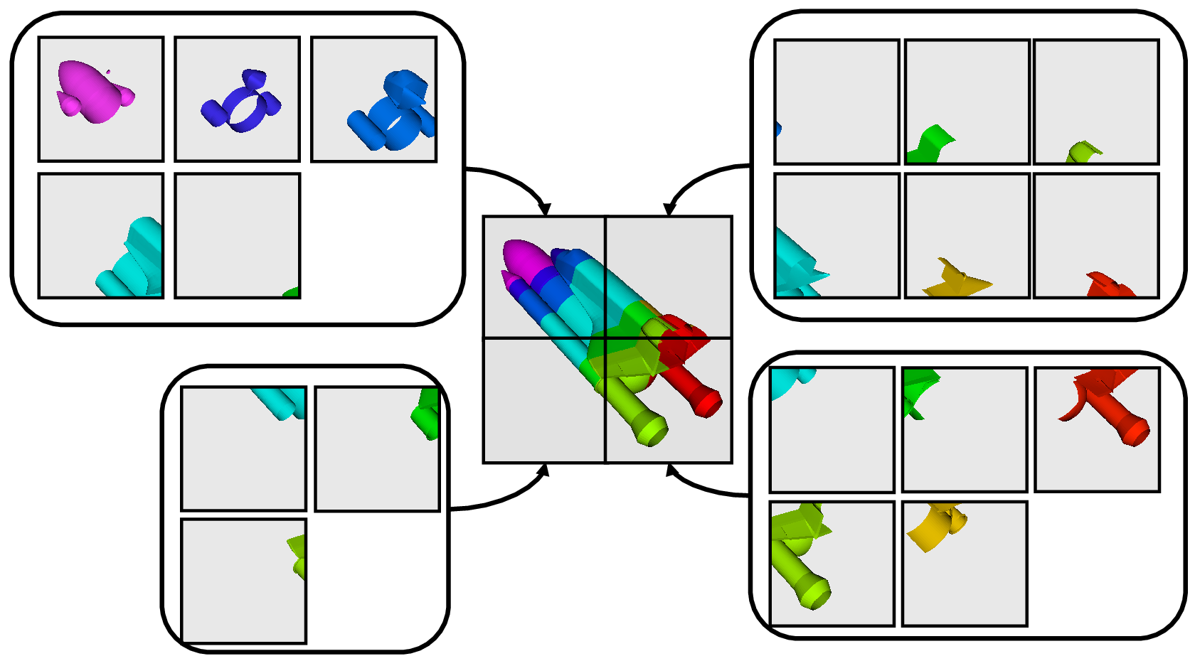
IceT also has the ability to drive tiled displays, which are large, high-resolution displays comprising an array of monitors or projectors. Using a sort-last algorithm on a tiled display is a bit counterintuitive because the number of pixels to composite is so large. However, IceT is designed to take advantage of spatial locality in the data on each process to drastically reduce the amount of compositing necessary. This spatial locality can be enforced by applying the Filters > Alphabetical > D3 filter to your data.
Because there is an overhead associated with parallel rendering, ParaView has the ability to turn off parallel rendering at any time. When parallel rendering is turned off, the geometry is shipped to the location where display occurs. Obviously, this should only happen when the data being rendered is small.
8.14.3. Image Level of Detail
The overhead incurred by the parallel rendering algorithms is proportional to the size of the images being generated. Also, images generated on a server must be transferred to the client, a cost that is also proportional to the image size. To help increase the frame rate during interaction, ParaView introduces a new LOD parameter that controls the size of the images.
During interaction while parallel rendering, ParaView can optionally subsample the image. That is, ParaView will reduce the resolution of the image in each dimension by a factor during interaction. Reduced images will be rendered, composited, and transferred. On the client, the image is inflated to the size of the available space in the GUI.
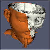
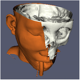
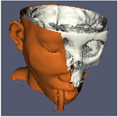

The resolution of the reduced images is controlled by the factor with which the dimensions are divided. In the proceeding images, the left image has the full resolution. The following images were rendered with the resolution reduced by a factor of 2, 4, and 8, respectively.
ParaView also has the ability to compress images before transferring them from server to client. Compression, of course, reduces the amount of data transferred and, therefore, makes the most of the available bandwidth. However, the time it takes to compress and decompress the images adds to the latency.
ParaView contains several different image compression algorithms for
client-server rendering. The first uses LZ4 compression that is designed
for high-speed compression and decompression. The second
option is a custom algorithm called
Squirt , which stands for Sequential Unified Image Run Transfer.
Squirt is a run-length encoding compression that reduces color depth to
increase run lengths. The third algorithm uses the Zlib
compression library, which implements a variation of the Lempel-Ziv
algorithm. Zlib typically provides better compression than Squirt, but
it takes longer to perform and, hence, adds to the latency. paraview Windows
and Linux executables include a compression option that uses NVIDIA’s
NVPipe library for hardware-accelerated compression and decompression if
a Kepler-class or higher NVIDIA GPU is available.
8.14.4. Parallel Render Parameters
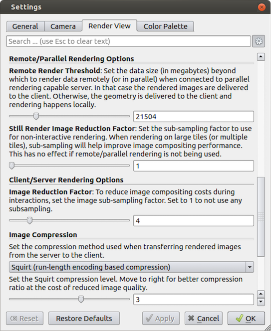
Like the other 3D rendering parameters, the parallel rendering parameters
are located in the Settings dialog.
The parallel rendering options in the dialog are in the
Render View tab (intermixed with several other rendering options such as those
described in Section 8.14.1). The parallel and
client-server options are divided among several categories, and several are
considered advanced.
Remote/Parallel Rendering OptionsRemote Render Threshold: Set the data size at which to render remotely in parallel or to render locally. If the geometry is over this threshold (and ParaView is connected to a remote server), the data is rendered in parallel remotely, and images are sent back to the client. If the geometry is under this threshold, the geometry is sent back to the client, and images are rendered locally on the client.Still Render Image Reduction Factor: Set the sub-sampling factor for still (non-interactive) rendering. Some large displays have more resolution than is really necessary, so this sub-sampling reduces the resolution of all images displayed.
Client/Server Rendering OptionsImage Reduction Factor: Set the interactive subsampling factor. The overhead of parallel rendering is proportional to the size of the images generated. Thus, you can speed up interactive rendering by specifying an image subsampling rate. When this box is checked, interactive renders will create smaller images, which are then magnified when displayed. This parameter is only used during interactive renders.
Image CompressionBefore images are shipped from server to client, they can optionally be compressed using one of three available compression algorithms: LZ4 , Squirt , or Zlib . To make the compression more effective, either algorithm can reduce the color resolution of the image before compression. The sliders determine the amount of color bits saved. Full color resolution is always used during a still render.
Suggested image compression presets are provided for several common network types. When attempting to select the best image compression options, try starting with the presets that best match your connection.
8.14.5. Parameters for Large Data
The default rendering parameters are suitable for most users. However, when dealing with very large data, it can help to tweak the rendering parameters. While the optimal parameters depend on your data and the hardware on which ParaView is running, here are several pieces of advice that you should follow.
If there is a long pause before the first interactive render of a particular dataset, it might be the creation of the decimated geometry. Try using an outline instead of decimated geometry for interaction. You could also try lowering the factor of the decimation to 0 to create smaller geometry.
Avoid shipping large geometry back to the client. The remote rendering will use the power of the entire server to render and ship images to the client. If remote rendering is off, geometry is shipped back to the client. When you have large data, it is always faster to ship images than to ship data. (Although, if your network has a high latency, this could become problematic for interactive frame rates.)
Adjust the interactive image sub-sampling for client-server rendering as needed. If image compositing is slow, if the connection between client and server has low bandwidth, or if you are rendering very large images, then a higher subsample rate can greatly improve your interactive rendering performance.
Make sure
Image Compressionis on. It has a tremendous effect on desktop delivery performance, and the artifacts it introduces, which are only there during interactive rendering, are minimal. Lower bandwidth connections can try using Zlib instead of Squirt compression. Zlib will create smaller images at the cost of longer compression/decompression times.If the network connection has a high latency, adjust the parameters to avoid remote rendering during interaction. In this case, you can try turning up the remote rendering threshold a bit, and this is a place where using the outline for interactive rendering is effective.
If the still (non-interactive) render is slow, try turning on the delay between interactive and still rendering to avoid unnecessary renders.