1. Introduction to ParaView
1.1. Introduction
ParaView is an open-source, multi-platform scientific data analysis and visualization tool that enables analysis and visualization of extremely large datasets. ParaView is both a general purpose, end-user application with a distributed architecture that can be seamlessly leveraged by your desktop or other remote parallel computing resources and an extensible framework with a collection of tools and libraries for various applications including scripting (using Python), web visualization (through ParaViewWeb), or in-situ analysis (with Catalyst).
ParaView leverages parallel data processing and rendering to enable interactive visualization for extremely large datasets. It also includes support for large displays including tiled displays and immersive 3D displays with head tracking and wand control capabilities.
ParaView also supports scripting and batch processing using Python. Using included Python modules, you can write scripts that can perform almost all the functionality exposed by the interactive application and much more.
ParaView is open-source (BSD licensed, commercial software friendly). As with any successful open-source project, ParaView is supported by an active user and developer community. Contributions to both the code and this user’s manual that help make the tool and the documentation better are always welcome.
Did you know?
The ParaView project started in 2000 as a collaborative effort between Kitware Inc. and LANL. The initial funding was provided by a three year contract with the US Department of Energy ASCI Views program. The first public release, ParaView 0.6, was announced in October 2002.
Independent of ParaView, Kitware started developing a web-based visualization system in December 2001. This project was funded by Phase I and II SBIRs from the US ARL and eventually became the PVEE. PVEE significantly contributed to the development of ParaView’s client/server architecture. PVEE was the precursor to ParaViewWeb, a modern web visualization solution based on ParaView.
Since the project began, Kitware has successfully collaborated with Sandia, LANL, the ARL, and various other academic and government institutions to continue development. Today, the project is still going strong!
In September 2005, Kitware, Sandia National Labs and CSimSoft started the development of ParaView 3.0. This was a major effort focused on rewriting the user interface to be more user friendly and on developing a quantitative analysis framework. ParaView 3.0 was released in May 2007.
1.1.1. In this guide
This user’s manual is designed as a guide for using the ParaView application. It is geared toward users who have a general understanding of common data visualization techniques. For scripting, a working knowledge of the Python language is assumed. If you are new to Python, there are several tutorials and guides for getting started that are available on the Internet.
Did You Know?
In this guide, we will periodically use these Did you know? boxes to provide additional information related to the topic at hand.
Common Errors
Common Errors blocks are used to highlight some of the common problems or complications you may run into when dealing with the topic of discussion.
This guide can be split into two volumes. Section 1 to Section 8 can be considered the user’s guide, where various aspects of data analysis and visualization with ParaView are covered. Section 1 to Section 11 in Reference manual part provide details on various components in the UI and the scripting API.
1.1.2. Getting help
This guide tries to cover most of the commonly used functionality in ParaView. ParaView’s flexible, pipeline-based architecture opens up numerous possibilities. If you find yourself looking for some feature not covered in this guide, refer to the Wiki pages (http://paraview.org/Wiki/ParaView) or to the forum (https://discourse.paraview.org/categories) specially the |FAQ| and the |Tips and Tricks| categories. Also feel free to ask about it under the relevant |Support| category.
1.1.3. Getting the software
ParaView is open source. The complete source code for all the functionality discussed in The ParaView Guide can be downloaded from the ParaView website http://www.paraview.org. We also provide binaries for the major platforms: Linux, Mac OS X, and Windows. You can get the source files and binaries for the official releases, as well as follow ParaView’s active development, by downloading the nightly builds.
Providing details of how to build ParaView using the source files is beyond the scope of this guide. Refer to the ParaView gitlab (https://gitlab.kitware.com/paraview/paraview/-/blob/master/Documentation/dev/build.md) for more information.
1.2. Basics of visualization in ParaView
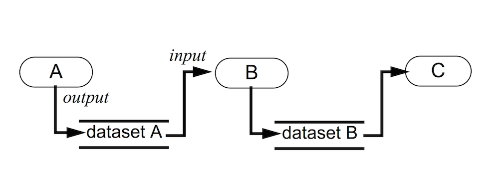
Fig. 1.1 Visualization model: Process objects A, B, and C input and/or output one or more data objects. Data objects represent and provide access to data; process objects operate on the data. Objects A, B, and C are source, filter, and mapper objects, respectively. [SML96]
Visualization is the process of converting raw data into images and renderings to gain a better cognitive understanding of the data. ParaView uses VTK, the Visualization Toolkit, to provide the backbone for visualization and data processing.
The VTK model is based on the data-flow paradigm. In this paradigm, data flows through the system being transformed at each step by modules known as algorithms. Algorithms could be common operations such as clipping, slicing, or generating contours from the data, or they could be computing derived quantities, etc. Algorithms have input ports through which they take in data and output ports through which they produce output. You need producers that ingest data into the system. These are simply algorithms that do not have an input port but have one or more output ports. They are called sources . Readers that read data from files are examples of such sources. Additionally, there are algorithms that transform the data into graphics primitives so that they can be rendered on a computer screen or saved to disk in another file. These algorithms, which have one or more input ports but do not have output ports, are called sinks . Intermediate algorithms with input ports and output ports are called filters . Together, sources, filters, and sinks provide a flexible infrastructure wherein you can create complex processing pipelines by simply connecting algorithms to perform arbitrarily complex tasks.
For more information on VTK’s programming model, refer to [SML96].
This way of looking at the visualization pipeline is at the core of ParaView’s work flow: You bring your data into the system by creating a reader – the source. You then apply filters to either extract information (e.g., iso-contours) and render the results in a view or to save the data to disk using writers – the sinks.
ParaView includes readers for a multitude of file formats typically used in the computational science world. To efficiently represent data from various fields with varying characteristics, VTK provides a rich data model that ParaView uses. The data model can be thought of simply as ways of representing data in memory. We will cover the different data types in more detail in Section 3.1. Readers produce a data type suitable for representing the information the files contain. Based on the data type, ParaView allows you to create and apply filters to transform the data. You can also show the data in a view to produce images or renderings. Just as there are several types of filters, each perfoming different operations and types of processing, there are several kinds of views for generating various types of renderings including 3D surface views, 2D bar and line views, parallel coordinate views, etc.
Did You Know?
The Visualization Toolkit (VTK) is an open-source, freely available software system for 3D computer graphics, modeling, image processing, volume rendering, scientific visualization, and information visualization. VTK also includes ancillary support for 3D interaction widgets, two and three-dimensional annotation, and parallel computing.
At its core, VTK is implemented as a C++ toolkit, requiring users to build applications by combining various objects into an application. The system also supports automated wrapping of the C++ core into Python, Java, and Tcl so that VTK applications may also be written using these interpreted programming languages. VTK is used world-wide in commercial applications, research and development, and as the basis of many advanced visualization applications such as ParaView, VisIt, VisTrails, Slicer, MayaVi, and OsiriX.
1.3. ParaView executables
ParaView comes with several executables that serve different purposes.
1.3.1. paraview
This is the main ParaView graphical user interface (GUI). In most cases, when we refer to ParaView, we are indeed talking about this application. It is a Qt-based, cross-platform UI that provides access to the ParaView computing capabilities. Major parts of this guide are dedicated to understanding and using this application.
1.3.2. pvpython
pvpython is the Python interpreter that
runs ParaView’s Python scripts. You can think of this as the equivalent of the
paraview for scripting.
1.3.3. pvbatch
Similar to pvpython, pvbatch is also a Python
interpreter that runs Python scripts for ParaView. The one difference is that, while
pvpython is meant to run interactive scripts, pvbatch
is designed for batch processing. Additionally, when running on computing
resources with MPI capabilities, pvbatch can be run in parallel. We
will cover this in more detail in Section 6.9.
1.3.4. pvserver
For remote visualization, this executable represents the server that does all
of the data processing and, potentially, the rendering.
You can make paraview connect to
pvserver running remotely on an HPC resource. This allows you to
build and control visualization and analysis on the HPC resource from your
desktop as if you were simply processing it locally on your desktop!
1.3.5. pvdataserver and pvrenderserver
These can be thought of as the pvserver split into two separate
executables: one for the data processing part, pvdataserver, and
one for the rendering part, pvrenderserver. Splitting these into
separate processes makes it possible to perform data processing and rendering on
separate sets of nodes with appropriate computing capabilities suitable for the
two tasks. Just as with pvserver, paraview can
connect to a pvdataserver- pvrenderserver pair for
remote visualization. Unless otherwise noted, all discussion of remote visualization or
client-server visualization in this guide is applicable to both
pvserver and pvdataserver - pvrenderserver configurations.
1.4. Getting started with paraview
1.4.1. paraview graphical user interface
paraview is the graphical front-end to the ParaView application. The
UI is designed to allow you to easily create pipelines for data processing with
arbitrary complexity. The UI provides panels for you to inspect and modify
the pipelines, to change parameters that in turn affect the processing pipelines,
to perform various data selection and inspection actions to introspect the data,
and to generate renderings. We will cover various aspects of the UI
for the better part of this guide.
Let’s start by looking at the various components of the UI. If you run
paraview for the first time, you will see something similar to the
Fig. 1.2. The UI is comprised of menus,
dockable panels, toolbars, and the viewport – the central portion of the
application window.
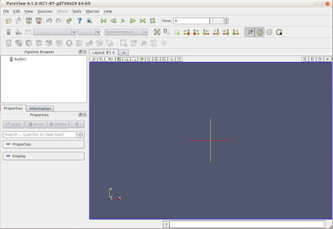
Fig. 1.2 paraview application window.
Menus provide the standard set of options typical with a desktop application
including options for opening/saving files (File
menu), for undo/redo (Edit menu), for the toggle panel, and for toolbar visibilities
(View menu). Additionally, the menus provide ways to create sources that
generate test datasets of various types (Sources menu), as well new
filters for processing data (Filters menu). The Tools menu
provides access to some of the advanced features in paraview such as
managing plugins and favorites.
Panels provide you with the ability to peek into the application’s state. For example, you can
inspect the visualization pipeline that has been set up ( Pipeline
Browser ), as well as the memory that is being used ( Memory Inspector ) and the parameters or properties
for a processing module ( Properties panel). Several of the panels also
allow you to change the values that are displayed, e.g., the Properties panel not only
shows the processing module parameters, but it also allows you to change them.
Several of the panels are context sensitive. For example, the Properties
panel changes to show the parameters from the selected module as you change the
active module in the Pipeline Browser .
Toolbars are designed to provide quick access to common functionality. Several of the actions in the toolbar are accessible from other locations, including menus or panels. Similar to panels, some of the toolbar buttons are context sensitive and will become enabled or disabled based on the selected module or view.
The viewport or the central portion of the paraview window is the
area where ParaView renders results generated from the data. The containers in
which data can be rendered or shown are called views. You can create
several different types of views, all of which are laid out in this viewport
area. By default, a 3D view is created, which is one of the most commonly used
views in ParaView.
1.4.2. Understanding the visualization process
To gain a better understanding of how to use the application interface, let’s consider a simple example: creating a data source and applying a filter to it.
1.4.3. Creating a source
The visualization process in ParaView begins by bringing your data into the application. Section 2 explains how to read data from various file formats. Besides reading files to bring in data into the application, ParaView also provides a collection of data sources that can produce sample datasets. These are available under the Sources menu. To create a source, simply click on any item in the Source menu.
Did You Know?
As you move your cursor over the items in any menu, on most platforms (except Mac OS X), you’ll see a brief description of the item in the status bar on the lower-left corner in the application window.
If you click on Sources > Sphere, for example, you’ll create a producer algorithm that generates a spherical surface, as shown in Fig. 1.3.
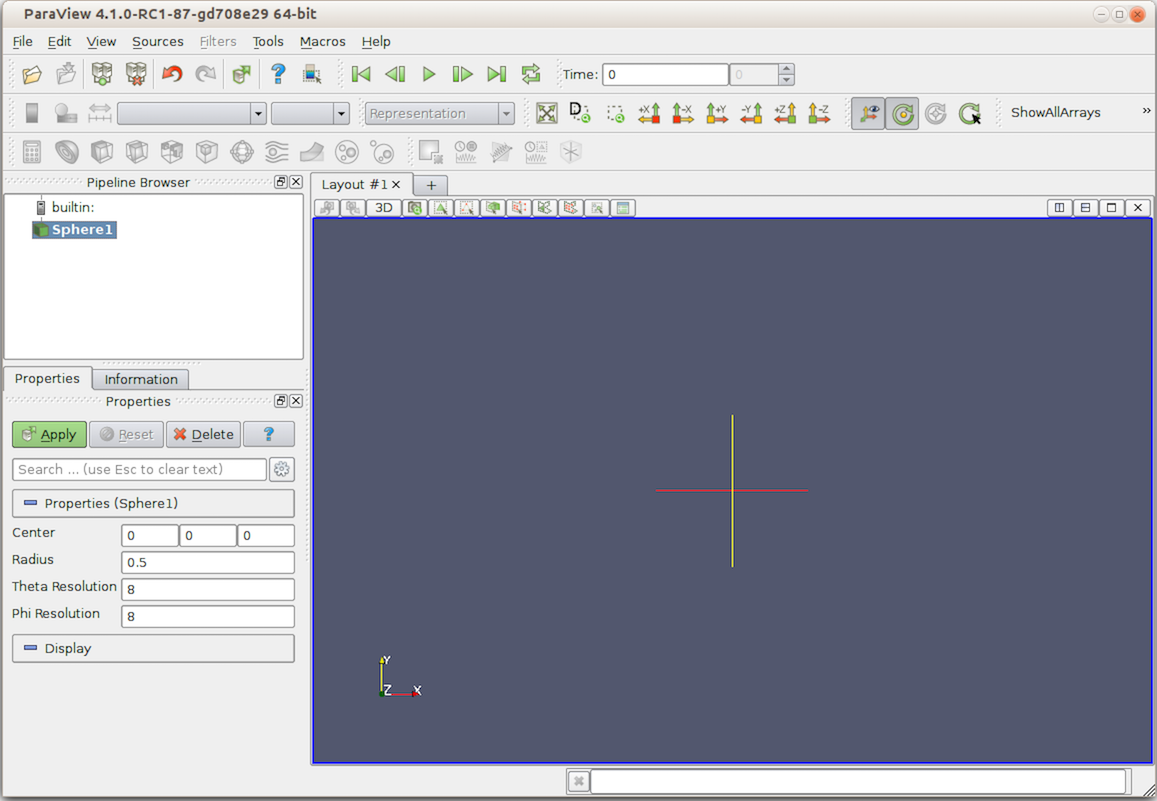
Fig. 1.3 Visualization in paraview: Step 1.
A few things to note:
A pipeline module is added in the
Pipeline Browserpanel with a name derived from the menu item, as is highlighted.The
Propertiespanel fills up with text to indicate that it’s showing properties for the highlighted item (which, in this case, isSphere1), as well as to display some widgets for parameters such asCenter,Radius, etc.On the
Propertiespanel, theApplybutton becomes enabled and highlighted.The 3D view remains unaffected, as nothing new is shown or rendered in this view as of yet.
Let’s take a closer look at what has happened. When we clicked on
Sources > Sphere, referring to
Section 1.2, we created an instance of a source that
can produce a spherical surface mesh – that’s what is reflected in the
Pipeline Browser .
This instance receives a name, which is used by the Sphere1 and the Pipeline Browser , as well as other
components of the UI, to refer to this instance of the source. Pipeline
modules such as sources and filters have parameters on them that you can change
that affect that module’s behavior. We call them properties. The
Properties panel shows these properties and allows you to change them.
Since the ingestion of data into the system can be a time-consuming process,
paraview allows you to change the properties before the module
executes or performs the actual processing to ingest the data. Hence, the
Apply button is highlighted to indicate that you need to accept the
properties before the application will proceed. Since no data has entered the
system yet, there’s nothing to show. Therefore, the 3D view remains unaffected.
Let’s assume we are okay with the default values for all of the properties on the
Sphere1 . Next, click on the Apply button.
Let’s assume we are okay with the default values for all of the properties on the
Sphere1. Next, click on the Apply button.
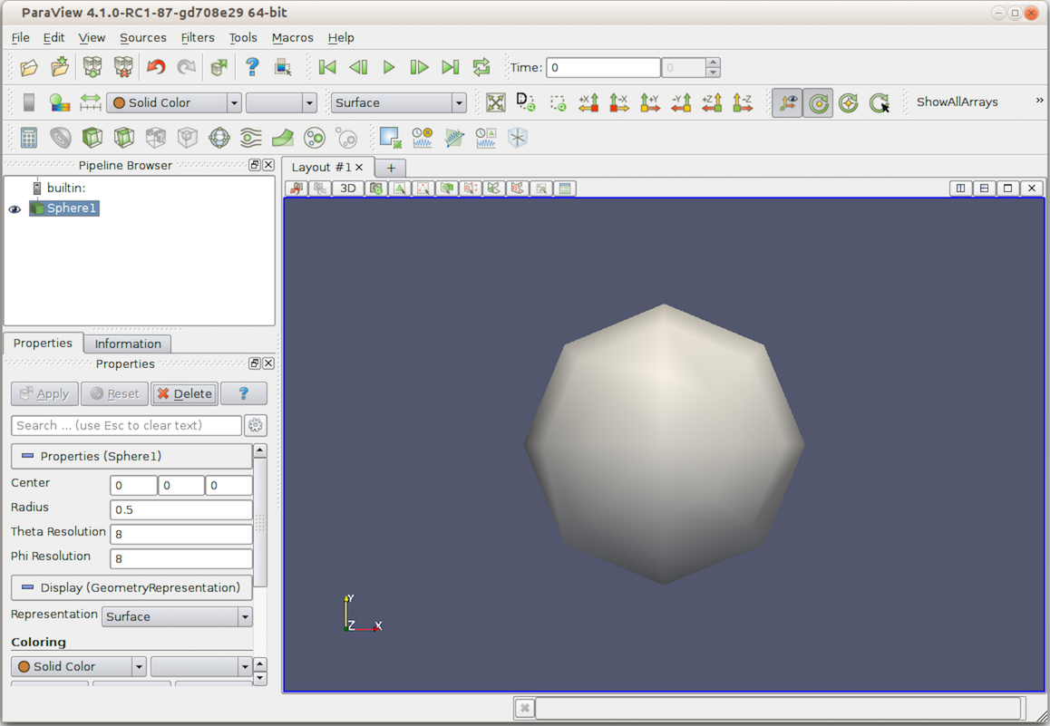
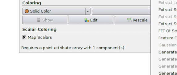
Fig. 1.4 Visualization in paraview: Step 2.
The following will ensue ( Fig. 1.4 ):
The
Applybutton goes back to its old disabled/un-highlighted state.A spherical surface is rendered in the 3D view.
The
Displaysection on thePropertiespanel now shows new parameters or properties.Certain toolbars update, and you can see that toolbars with text, such as
Solid ColorandSurface, now become enabled.
By clicking Apply , we told paraview to apply the properties
shown on the Properties panel. When a new source (or filter) is
applied for the first time, paraview will automatically show
the data that the pipeline module produces in the current view, if possible.
In this case, the sphere source produces a surface mesh, which is then shown or
displayed in the 3D view.
The properties that allow you to control how
the data is displayed in the view are now shown on the Properties panel in
the Display section. Things such as the surface color, rendering type or
representation, shading parameters, etc., are shown under this newly updated
section. We will look at display properties in more detail in
Section 4.
Some of the properties that are commonly used are also duplicated in the toolbar. These properties include the data array with which the surface is colored and the representation type. These are the changes in the toolbar that allow you to quickly change some display properties.
1.4.4. Changing properties
If you change any of the properties on the sphere source, such as the properties
under the Properties
section on the Properties panel, including the Radius
for the spherical mesh or its Center , the Apply button will be
highlighted again. Once you are finished with all of the property changes, you can
hit Apply to apply the changes. Once the changes are applied,
paraview will re-execute the sphere source to produce a new mesh,
as requested. It will then automatically update the view, and you will see the
new result rendered.
If you change any of the display properties for the sphere source, such as the
properties under the Display section of the Properties panel (including
Representation or Opacity ), the Apply button is not affected, the
changes are immediately applied, and the view is updated.
The rationale behind this is that, typically, the execution of the source (or filter) is more computationally intensive than the rendering. Changing source (or filter) properties causes that algorithm to re-execute, while changing display properties, in most cases, only triggers a fresh render with an updated graphics state.
Did You Know?
For some workflows with smaller data sizes, it may be more convenient
if the Apply button was automatically applied even after changes are made to the
pipeline module properties. You can change this from the application settings dialog, which is
accessible from the Edit > Settings menu. The setting is called Auto Apply .
You can also change the Auto Apply state using the
 button from the toolbar.
1.4.5. Applying filters
As per the data-flow paradigm, one creates pipelines with filters to transform data. Similar to the Sources menu, which allows us to create new data sources, there’s a Filters menu that provides access to the large set of filters that are available in ParaView. If you peruse the items in this menu, some of them will be enabled, and some of them will be disabled. Filters that can work with the data type being produced by the sphere source are enabled, while others are disabled. You can click on any of the enabled filters to create a new instance of that filter type.
Did You Know?
To figure out why a particular filter doesn’t work with the current source, simply move your mouse over the disabled item in the Filters menu. On Linux and Windows (not OS X, however), the status bar will provide a brief explanation of why that filter is not available.
For example, if you click on Filters > Shrink, it will create a filter
that shrinks each of the mesh cells by a fixed factor. Exactly as before, when we
created the sphere source, we see that the newly-created filter is given a new
name, Shrink1 , and is highlighted in the Pipeline Browser . The
Properties panel is also updated to show the properties for this new
filter, and the Apply button is highlighted to request that we accept the
properties for the filter so that it can be executed and the result can be rendered. If you
click back and forth between the Sphere1 and Shrink1 in the
Pipeline Browser , you’ll see the Properties panel and toolbars update,
reflecting the state of the selected pipeline module. This is an important
concept in ParaView. There’s a notion of active pipeline module, called the
active source .
Several panels, toolbars, and menus will update based on
the active source.
If you click Apply , as was the case before, the shrink filter will be executed and the
resulting dataset will be generated and shown in the 3D view. paraview
will also automatically hide the result from the Sphere1 so that it is not shown
in the view. Otherwise, the two datasets will overlap. This is reflected by
the change of state for the eyeball icons in the Pipeline Browser
next to each of the pipeline modules. You can show or hide results from any
pipeline module by clicking on the eyeballs.
This simple workflow forms the basis of all the data analysis and visualization in ParaView. The process involves creating sources and filters, changing their parameters, and showing the generated result in one or more views. In the rest of this guide, we will cover various types of filters and data processing that you can do. We will also cover different types of views that can help you produce a wide array of 2D and 3D visualizations, as well as inspect your data and drill down into it.
Common Errors
Beginners often forget to hit the Apply button after creating sources or
filters or after changing properties. This is one of the most common pitfalls for
users new to the ParaView workflow.
1.5. Getting started with pvpython
While this section refers to pvpython, everything that we discuss
here is applicable to pvbatch as well. Until we start looking into
parallel processing, the only difference between the two executables is that
pvpython provides an interactive shell wherein you can type your
commands, while pvbatch expects the Python script to be specified
on the command line argument.
1.5.1. pvpython scripting interface
ParaView provides a scripting interface to write scripts for performing the tasks that you could do using the GUI. The scripting interface can be accessed through Python, which is an interpreted programming language popular among the scientific community for its simplicity and its capabilities. While a working knowledge of Python will be useful for writing scripts with advanced capabilities, you should be able to follow most of the discussion in this book about ParaView scripting even without much Python exposure.
ParaView provides a paraview package with several Python modules that expose
various functionalities. The primary scripting interface is provided by the
simple module.
When you start pvpython, you should see a prompt in a terminal
window as follows (with some platform specific differences).
Python 2.7.5 (default, Sep  2 2013, 05:24:04)
[GCC 4.2.1 Compatible Apple LLVM 5.0 (clang-500.0.68)] on darwin
Type "help", "copyright", "credits" or "license" for more information
>>>
You can now type commands at this prompt, and ParaView will execute them. To
bring in the ParaView scripting API, you first need to import the simple
module from the paraview package as follows:
>>> from paraview.simple import *
Common Errors
Remember to hit the Enter or Return key after every command to execute
it. Any Python interpreter will not execute the command until Enter is hit.
If the module is loaded correctly, pvpython will present a prompt for the next
command.
>>> from paraview.simple import *
>>>
You can consider this as in the same state as when paraview was
started (with some differences that we can ignore for now). The application is
ready to ingest data and start processing.
1.5.2. Understanding the visualization process
Let’s try to understand the workflow by looking at the same use-case as we did in Section 1.4.2.
1.5.3. Creating a source
In paraview, we created the data source by using the Sources
menu. In the scripting environment, this maps to simply typing the name of the
source to create.
>>> Sphere()
This will create the sphere source with a default set of properties. Just like
with paraview, as soon as a new pipeline module is created, it
becomes the active source.
Now, to show the active source in a view, try:
>>> Show()
>>> Render()
The Show call will prepare the display, while the Render call will
cause the rendering to occur. In addition, a new window will popup, showing the result
(Fig. 1.5). This is similar to the state after hitting
Apply in the UI.
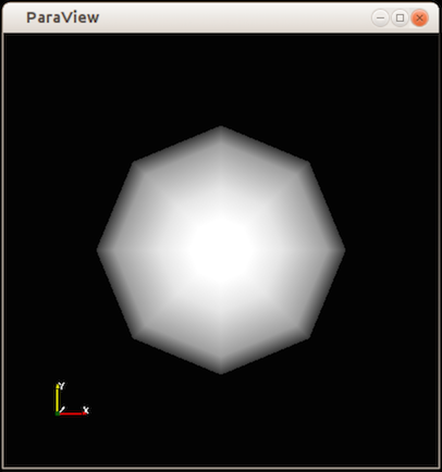
Fig. 1.5 Window showing result from the Python code.
1.5.4. Changing properties
To change the properties on the sphere source, you can use the SetProperties
function.
# Set a single property on the active source.
>>> SetProperties(Radius=1.0)

# You can also set multiple properties.
>>> SetProperties(Center=[1, 0, 0], StartTheta=100)
Similar to the Properties panel, SetProperties affects the active
source. To query the current value of any property on the active source, use
GetProperty .
>>> radius = GetProperty("Radius")
>>> print(radius)
1.0
>>> center = GetProperty("Center")
>>> print(center)
[1.0, 0.0, 0.0]
SetProperties and GetProperty functions serve the same function as the
Properties section of the Properties panel – they allow you to set
and introspect the pipeline module properties for the active source.
Likewise, for the Display section of the panel, or the display properties,
we have the SetDisplayProperties and GetDisplayProperty functions.
>>> SetDisplayProperties(Opacity=0.5)
>>> GetDisplayProperty("Opacity")
0.5
Common Errors
Note how the property names for the SetProperties and
SetDisplayProperties functions are not enclosed in double-quotes, while
those for the GetProperty and GetDisplayProperty methods are.
In paraview, every time you hit Apply or change a display
property, the UI automatically re-renders the view. In the scripting environment,
you have to do this manually by calling the Render function every time you want
to re-render and look at the updated result.
fixme{we’re missing blurb about reset camera}.
1.5.5. Applying filters
Similar to creating a source, to apply a filter, you can simply create the filter by name.
# Create the `Shrink' filter and connect it to the active source
# which is the `Sphere' instance.
>>> Shrink()
# As soon as the Shrink filter is created, it will now become the new active
# source. All methods acting on active source now act on this filter instance
# and not the Sphere instance created earlier.

# Show the resulting data and render it.
>>> Show()
>>> Render()
If you tried the above script, you’ll notice the result isn’t exactly what we
expected. For some reason, the shrank cells are not visible. This is because we
missed one stage: In paraview, the UI was smart enough to
automatically hide the input dataset for the newly created filter after we hit
apply. In the scripting interface, such operations are the user’s responsibility. We
should have hidden the sphere source from the view. We can use the Hide
method, the counter part of Show , to hide the active source. But, now we have
a problem – when we created the shrink filter, we changed the active source to
be the shrink instance. Luckily, all the functions we discussed so far can take
an optional first argument, which is the source or filter instance on which to operate.
If provided, that instance is used instead of the active source.
The solution is as follows:
# Get the input property for the active source, i.e. the input for the shrink.
>>> shrinksInput = GetProperty("Input")

# This is indeed the sphere instance we created earlier.
>>> print(shrinksInput)
<paraview.servermanager.Sphere object at 0x11d731e90>

# Hide the sphere instance explicitly.
>>> Hide(shrinksInput)

# Re-render the result.
>>> Render()
Alternatively, you could also get/set the active source using the GetActiveSource and SetActiveSource functions.
>>> shrinkInstance = GetActiveSource()
>>> print(shrinkInstance)
<paraview.servermanager.Shrink object at 0x11d731ed0>

# Get the input property for the active source, i.e. the input
# for the shrink.
>>> sphereInstance = GetProperty("Input")

# This is indeed the sphere instance we created earlier.
>>> print(sphereInstance)
<paraview.servermanager.Sphere object at 0x11d731e90>

# Change active source to sphere and hide it.
>>> SetActiveSource(sphereInstance)
>>> Hide()

# Now restore the active source back to the shrink instance.
>>> SetActiveSource(shrinkInstance)

# Re-render the result
>>> Render()
The result is shown in Fig. 1.6 .
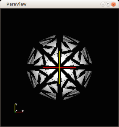
Fig. 1.6 Window showing result from the Python code after applying the shrink filter.
SetActiveSource has same effect as changing
the pipeline module, highlighted in the Pipeline Browser ,
by clicking on a different module.
1.5.6. Alternative approach
Here’s another way of doing something similar to what we did in the previous section for those familiar with Python and/or object-oriented programming. It’s totally okay to stick with the previous approach.
>>> from paraview.simple import *
>>> sphereInstance = Sphere()
>>> sphereInstance.Radius = 1.0
>>> sphereInstance.Center[1] = 1.0
>>> print(sphereInstance.Center)
[0.0, 1.0, 0.0]

>>> sphereDisplay = Show(sphereInstance)
>>> view = Render()
>>> sphereDisplay.Opacity = 0.5

# Render function can take in an optional view argument, otherwise it
# will simply use the active view.
>>> Render(view)

>>> shrinkInstance = Shrink(Input=sphereInstance,
                            ShrinkFactor=1.0)
>>> print(shrinkInstance.ShrinkFactor)
1.0
>>> Hide(sphereInstance)
>>> shrinkDisplay = Show(shrinkInstance)
>>> Render()
1.5.7. Updating the pipeline
When changing properties on the Properties panel in
paraview, we noticed that the algorithm doesn’t re-execute until
you hit Apply . In reality, Apply isn’t what’s actually triggering
the execution or the updating of the processing pipeline. What happens is that
Apply updates the parameters on the pipeline module and causes the view to
render. If the output of the pipeline module is visible in the view, or if the output of
any filter connected to it downstream is visible in the view, ParaView will
determine that the data rendered is obsolete and request the pipeline to
re-execute. It implies that if that pipeline module (or any of the filters
downstream from it) is not visible in the view, ParaView will have no reason to
re-execute the pipeline, and the pipeline module will not be be updated. If, later
on, you do make this module visible in the view, ParaView will automatically
update and execute the pipeline. This is often referred to as
demand-driven pipeline execution . It makes it possible to avoid unnecessary module executions.
In paraview, you can get by without ever noticing this since the
application manages pipeline updates automatically. In pvpython
too, if your scripts are producing renderings in views, you’d never
notice this as long as you remember to call Render . However, you may want
to write scripts to produce transformed datasets or to determine data
characteristics. In such cases, since you may never create a view, you’ll never
be seeing the pipeline update, no matter how many times you change the
properties.
Accordingly, you must use the UpdatePipeline function.
UpdatePipeline updates the pipeline connected to the active source (or only
until the active source, i.e., anything downstream from it, won’t be updated).
>>> from paraview.simple import *
>>> sphere = Sphere()

# Print the bounds for the data produced by sphere.
>>> print(sphere.GetDataInformation().GetBounds())
(1e+299, -1e+299, 1e+299, -1e+299, 1e+299, -1e+299)
# The bounds are invalid -- no data has been produced yet.

# Update the pipeline explicitly on the active source.
>>> UpdatePipeline()

# Alternative way of doing the same but specifying the source
# to update explicitly.
>>> UpdatePipeline(proxy=sphere)

# Let's check the bounds again.
>>> sphere.GetDataInformation().GetBounds()
(-0.48746395111083984, 0.48746395111083984, -0.48746395111083984, 0.48746395111083984, -0.5, 0.5)

# If we call UpdatePipeline() again, this will have no effect since
# the pipeline hasn't been modified, so there's no need to re-execute.
>>> UpdatePipeline()
>>> sphere.GetDataInformation().GetBounds()
(-0.48746395111083984, 0.48746395111083984, -0.48746395111083984, 0.48746395111083984, -0.5, 0.5)

# Now let's change a property.
>>> sphere.Radius = 10

# The bounds won't change since the pipeline hasn't re-executed.
>>> sphere.GetDataInformation().GetBounds()
(-0.48746395111083984, 0.48746395111083984, -0.48746395111083984, 0.48746395111083984, -0.5, 0.5)

# Let's update and see:
>>> UpdatePipeline()
>>> sphere.GetDataInformation().GetBounds()
(-9.749279022216797, 9.749279022216797, -9.749279022216797, 9.749279022216797, -10.0, 10.0)
We will look at the sphere.GetDataInformation API in
Section 3.3 in more detail.
For temporal datasets, UpdatePipeline takes in a time argument, which is the
time for which the pipeline must be updated.
# To update to time 10.0:
>>> UpdatePipeline(10.0)

# Alternative way of doing the same:
>>> UpdatePipeline(time=10.0)

# If not using the active source:
>>> UpdatePipeline(10.0, source)
>>> UpdatePipeline(time=10.0, proxy=source)
1.6. Scripting in paraview
1.6.1. The Python Shell
The paraview application also provides access to an internal shell, in which
you can enter Python commands and scripts exactly as with
pvpython. To access the Python shell in the GUI, use the
View > Python Shell menu option. A dialog will pop up with a
prompt exactly like pvpython. You can try inputting commands from
the earlier section into this shell. As you type each of the commands, you will
see the user interface update after each command, e.g., when you create the
sphere source instance, it will be shown in the Pipeline Browser . If you
change the active source, the Pipeline Browser and other UI components will
update to reflect the change. If you change any properties or display properties, the
Properties panel will update to reflect the change as well!
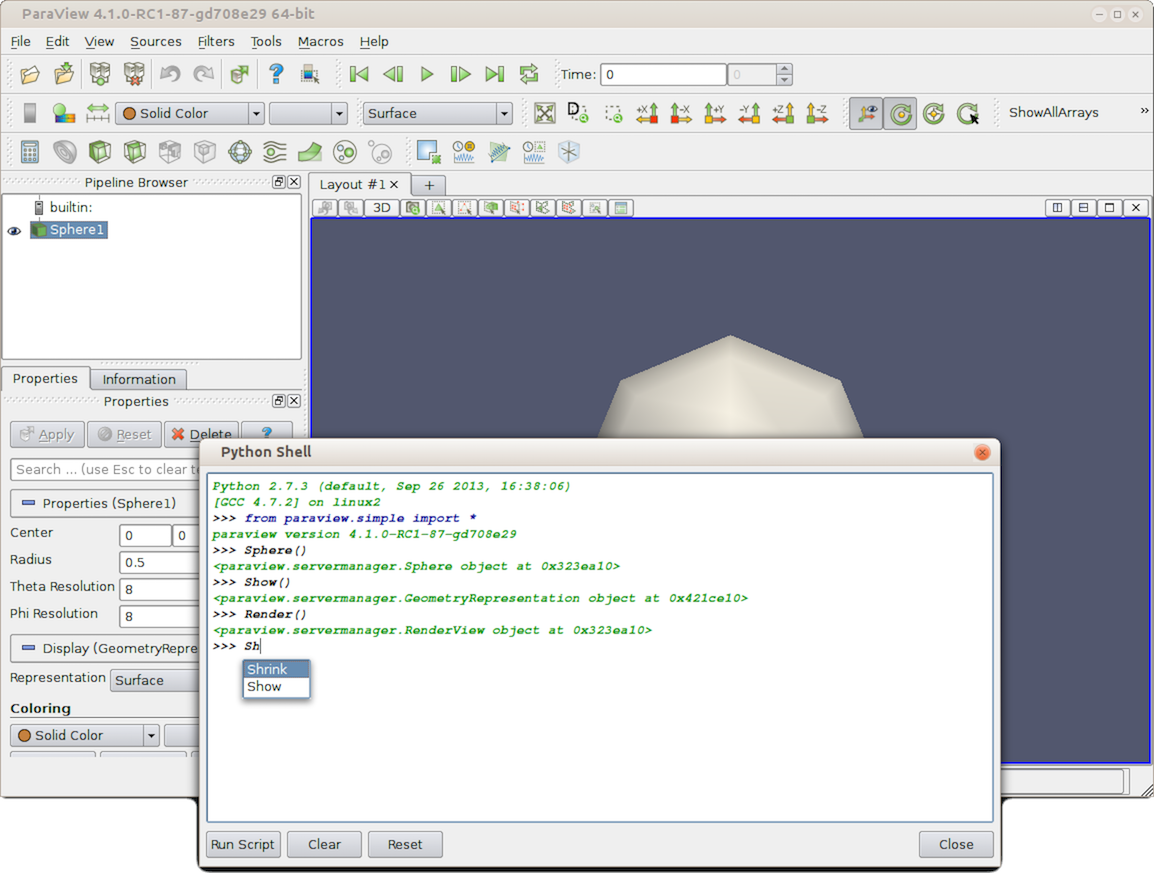
Fig. 1.7 Python Shell in paraview provides access to the scripting.
Did You Know?
The Python Shell in paraview supports auto-completion for functions
and instance methods. Try hitting the Tab key after partially typing any
command (as shown in Fig. 1.7).
1.6.2. Tracing actions for scripting
This guide provides a fair overview of ParaView’s Python API. However, there
will be cases when you just want to know how to complete a particular action or
sequence of actions that you can do with the GUI using a Python script instead. To
accomplish this, paraview supports tracing your actions in
the UI as a Python script. Simply start tracing by clicking on
Tools > Start Trace. paraview now enters a mode where all
your actions (or at least those relevant for scripting) are monitored. Any time
you create a source or filter, open data files,
change properties and hit Apply , interact with the 3D scene, or save
screenshots, etc., your actions will be monitored. Once you are done with the series of
actions that you want to script, click
Tools > Stop Trace. paraview will then pop up an editor
window with the generated trace. This will be the Python script equivalent for
the actions you performed. You can now save this as a script to use for batch
processing.