4. Programmable Filter
A pipeline module in ParaView does one of two things: it either generates data or processes input data. To generate data, the module may use a mathematical model e.g. Sources > Sphere or read a file from disk. Processing data entails transforming input data by applying defined operations to generate a new output. ParaView provides a large set of readers, data sources and data filters that cover the needs of many users. For the cases where the available collection does not satisfy your needs, ParaView provides a mechanism to add new modules via plugins. Conventional plugins, however, are intended for hardcore developers. They are written in C++, using the data processing APIs provided by ParaView and VTK. The complexity of building and packaging C++ plugins that work on all distributed versions of ParaView can be daunting and thus a huge barrier for even advanced ParaView users. Python-based programmable filters and sources provide an easy alternative to this. New modules can be written as Python scripts that are executed by ParaView to generate and/or process data, just like conventional C++ modules. Since the scripts are standard Python scripts, you have access to Python packages such as NumPy that provide several numeric operations useful for data transformation.
In this chapter, we will explore how to use Python to add new data processing modules to ParaView through examples. For additional explanation of the data processing API, see Section 5.
Common Errors
In this guide so far, we have been looking at examples of Python scripts for
pvpython. These scripts are used to script the actions you would
perform using the paraview UI. The scripts you would
write for Programmable Source and Programmable Filter are entirely
different. The data processing API executes within the data processing
pipeline and, thus, has access to the data being processed. In client-server
mode, this means that such scripts are indeed executed on the server side,
potentially in parallel, across several MPI ranks. Therefore, attempting to import
the paraview.simple Python module in the Programmable Source script, for
example, is not supported and will have unexpected consequences.
4.1. Understanding the programmable modules
With programmable modules, you are writing custom code for filters and sources. You are expected to understand the basics of a VTK (and ParaView) data processing pipeline, including the various stages of the pipeline execution as well as the data model. Refer to Section 3.1 for an overview of the VTK data model. While a detailed discussion of the VTK pipeline execution model is beyond the scope of this book, the fundamentals covered in this section, along with the examples in the rest of this chapter, should help you get started and write useful modules. For a primer on the details of the VTK pipeline execution stages, see [BerkGeveci].
To create the programmable source or filter in paraview,
you use the Sources > Programmable Source or Filters > Programmable Filter
menus, respectively. Since the Programmable Filter is a filter,
like other filters, it gets connected to the currently active source(s), i.e., the
currently active source(s) become the input to this new filter. Programmable
Source , on the other hand, does not have any inputs.
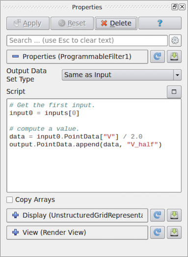
Fig. 4.19 Properties panel for Programmable Filter in paraview.
One of the first things that you specify after creating any of these programmable
modules is the Output Data Set Type . This option lets you select the type
of dataset this module will produce. The options provided include several of the
data types discussed in Section 3.1. Additionally, for the
Programmable Filter , you can select Same as Input to indicate that
the filter preserves the input dataset type.
Next is the primary part: the Script . This is where you enter the Python
script to generate or process from the inputs the dataset that the module will
produce. As with any Python script, you can import other Python packages and
modules in this script. Just be aware that when running in client-server mode,
this script is going to be executed on the server side. Accordingly, any modules or
packages you import must be available on the server side to avoid errors.
The script gets executed in what’s called the RequestData pass of the pipeline execution. This is the pipeline pass in which an algorithm is expected to produce the output dataset.
There are several other passes in a pipeline’s execution. The ones for which you can specify a Python script to execute with these programmable modules are:
RequestInformation: In this pass, the algorithm is expected to provide the pipeline with any meta-data available about the data that will be produced by it. This includes things like number of timesteps in the dataset and their time values for temporal datasets or extents for structured datasets. This gets called before RequestData pass. In the RequestData pass, the pipeline could potentially qualify the request based on the meta-data provided in this pass. For example, if an algorithm announces that the temporal dataset has multiple timesteps, the pipeline could request that the algorithm produce data for one of those timesteps in
RequestData.RequestUpdateExtent: In this pass, a filter gets the opportunity to qualify requests for execution passed on to the upstream pipeline. As an example, if an upstream reader announced in its RequestInformation script that it can produce several timesteps, in RequestUpdateExtent, this filter can make a request to the upstream reader for a specific timestep. This pass gets called after RequestInformation, but before
RequestData. It’s not very common to provide a script for this pass.
You can specify the script for the RequestInformation pass in
RequestInformation Script and for the RequestUpdateExtent pass in
RequestUpdateExtent Script . Since the RequestUpdateExtent pass does not make
much sense for an algorithm that does not have any inputs, RequestUpdateExtent Script
is not available on Programmable Source .
4.2. Recipes for Programmable Source
In this section, we look at several recipes for Programmable Source . A
common use of Programmable Source is to prototype readers. If your reader
library already provides a Python API, then you can easily import the
appropriate Python package to read your dataset using Programmable Source .
Did you know?
Most of the examples in this chapter use a NumPy-centric API for accessing and creating data arrays. Additionally, you can use VTK’s Python wrapped API for creating and accessing arrays. Given the omnipresence of NumPy, there is rarely any need for using VTK’s API directly, however.
4.2.1. Reading a CSV file
For this example, we will read in a CSV file to produce a Table
( Section 3.1.9) using Programmable Source . We will
use NumPy to do the parsing of the CSV files and pass the arrays read in
directly to the pipeline. Note that the Output DataSet Type must be set
to vtkTable .
# Code for 'Script'
# We will use NumPy to read the csv file.
# Refer to NumPy documentation for genfromtxt() for details on
# customizing the CSV file parsing.
import numpy as np
# assuming data.csv is a CSV file with the 1st row being the names names for
# the columns
data = np.genfromtxt("data.csv", dtype=None, names=True, delimiter=',', autostrip=True)
for name in data.dtype.names:
array = data[name]
# You can directly pass a NumPy array to the pipeline.
# Since ParaView expects all arrays to be named, you
# need to assign it a name in the 'append' call.
output.RowData.append(array, name)
4.2.2. Reading a CSV file series
Building on the example from Section 4.2.1,
let’s say we have a series of files that we
want to read in as a temporal series. Recall from
Section 4.1 that meta-data about data to
be produced, including timestep information, is announced in
RequestInformation pass. Hence, for this example, we will need to specify
the RequestInformation Script as well.
As was true earlier, Output DataSet Type must be set to vtkTable .
Now, to announce the timesteps, we use the following as the
RequestInformation Script .
# Code for 'RequestInformation Script'.
def setOutputTimesteps(algorithm, timesteps):
"helper routine to set timestep information"
executive = algorithm.GetExecutive()
outInfo = executive.GetOutputInformation(0)
outInfo.Remove(executive.TIME_STEPS())
for timestep in timesteps:
outInfo.Append(executive.TIME_STEPS(), timestep)
outInfo.Remove(executive.TIME_RANGE())
outInfo.Append(executive.TIME_RANGE(), timesteps[0])
outInfo.Append(executive.TIME_RANGE(), timesteps[-1])
# As an example, let's say we have 4 files in the file series that we
# want to say are producing time 0, 10, 20, and 30.
setOutputTimesteps(self, (0, 10, 20, 30))
The Script is similar to earlier, except that we will read a specific
CSV file based on which timestep was requested.
# Code for 'Script'
def GetUpdateTimestep(algorithm):
"""Returns the requested time value, or None if not present"""
executive = algorithm.GetExecutive()
outInfo = executive.GetOutputInformation(0)
return outInfo.Get(executive.UPDATE_TIME_STEP()) \
if outInfo.Has(executive.UPDATE_TIME_STEP()) else None
# This is the requested time-step. This may not be exactly equal to the
# timesteps published in RequestInformation(). Your code must handle that
# correctly.
req_time = GetUpdateTimestep(self)
# Now, use req_time to determine which CSV file to read and read it as before.
# Remember req_time need not match the time values put out in
# 'RequestInformation Script'. Your code need to pick an appropriate file to
# read, irrespective.
...
# TODO: Generate the data as you want.
# Now mark the timestep produced.
output.GetInformation().Set(output.DATA_TIME_STEP(), req_time)
4.2.3. Reading a CSV file with particles
This is similar to Section 4.2.1. Now, however, let’s say the CSV has three
columns named X, Y and Z that we want to treat as point coordinates and
produce a vtkPolyData with points instead of a vtkTable . For that, we first
ensure that Output DataSet Type is set to vtkPolyData . Next, we use
the following Script :
# Code for 'Script'
from vtk.numpy_interface import algorithms as algs
from vtk.numpy_interface import dataset_adapter as dsa
import numpy as np
# assuming data.csv is a CSV file with the 1st row being the names names for
# the columns
data = np.genfromtxt("/tmp/points.csv", dtype=None, names=True, delimiter=',', autostrip=True)
# convert the 3 arrays into a single 3 component array for
# use as the coordinates for the points.
coordinates = algs.make_vector(data["X"], data["Y"], data["Z"])
# create a vtkPoints container to store all the
# point coordinates.
pts = vtk.vtkPoints()
# numpyTovtkDataArray is needed to called directly to convert the NumPy
# to a vtkDataArray which vtkPoints::SetData() expects.
pts.SetData(dsa.numpyTovtkDataArray(coordinates, "Points"))
# set the pts on the output.
output.SetPoints(pts)
# next, we define the cells i.e. the connectivity for this mesh.
# here, we are creating merely a point could, so we'll add
# that as a single poly vextex cell.
numPts = pts.GetNumberOfPoints()
# ptIds is the list of point ids in this cell
# (which is all the points)
ptIds = vtk.vtkIdList()
ptIds.SetNumberOfIds(numPts)
for a in xrange(numPts):
ptIds.SetId(a, a)
# Allocate space for 1 cell.
output.Allocate(1)
output.InsertNextCell(vtk.VTK_POLY_VERTEX, ptIds)
# We can also pass all the array read from the CSV
# as point data arrays.
for name in data.dtype.names:
array = data[name]
output.PointData.append(array, name)
The thing to note is that this time, we need to define the geometry and topology for the output dataset. Each data type has different requirements on how these are specified. For example, for unstructured datasets like vtkUnstructuredGrid and vtkPolyData, we need to explicitly specify the geometry and all the connectivity information. For vtkImageData, the geometry is defined using origin, spacing, and extents, and connectivity is implicit.
4.2.4. Reading binary 2D image
This recipe shows how to read raw binary data representing a 3D volume. Since raw binary files don’t encode information about the volume extents and data type, we will assume that the extents and data type are known and fixed.
For producing image volumes, you need to provide the information about the
structured extents in RequestInformation. Ensure that the Output
Data Set Type is set to vtkImageData .
# Code for 'RequestInformation Script'.
executive = self.GetExecutive()
outInfo = executive.GetOutputInformation(0)
# we assume the dimensions are (48, 62, 42).
outInfo.Set(executive.WHOLE_EXTENT(), 0, 47, 0, 61, 0, 41)
outInfo.Set(vtk.vtkDataObject.SPACING(), 1, 1, 1)
The Script to read the data can be written as follows.
# Code for 'Script'
import numpy as np
# read raw binary data.
# ensure 'dtype' is set properly.
data = np.fromfile("HeadMRVolume.raw", dtype=np.uint8)
dims = [48, 62, 42]
assert data.shape[0] == dims[0]*dims[1]*dims[2], "dimension mismatch"
output.SetExtent(0, dims[0]-1, 0, dims[1]-1, 0, dims[2]-1)
output.PointData.append(data, "scalars")
output.PointData.SetActiveScalars("scalars")
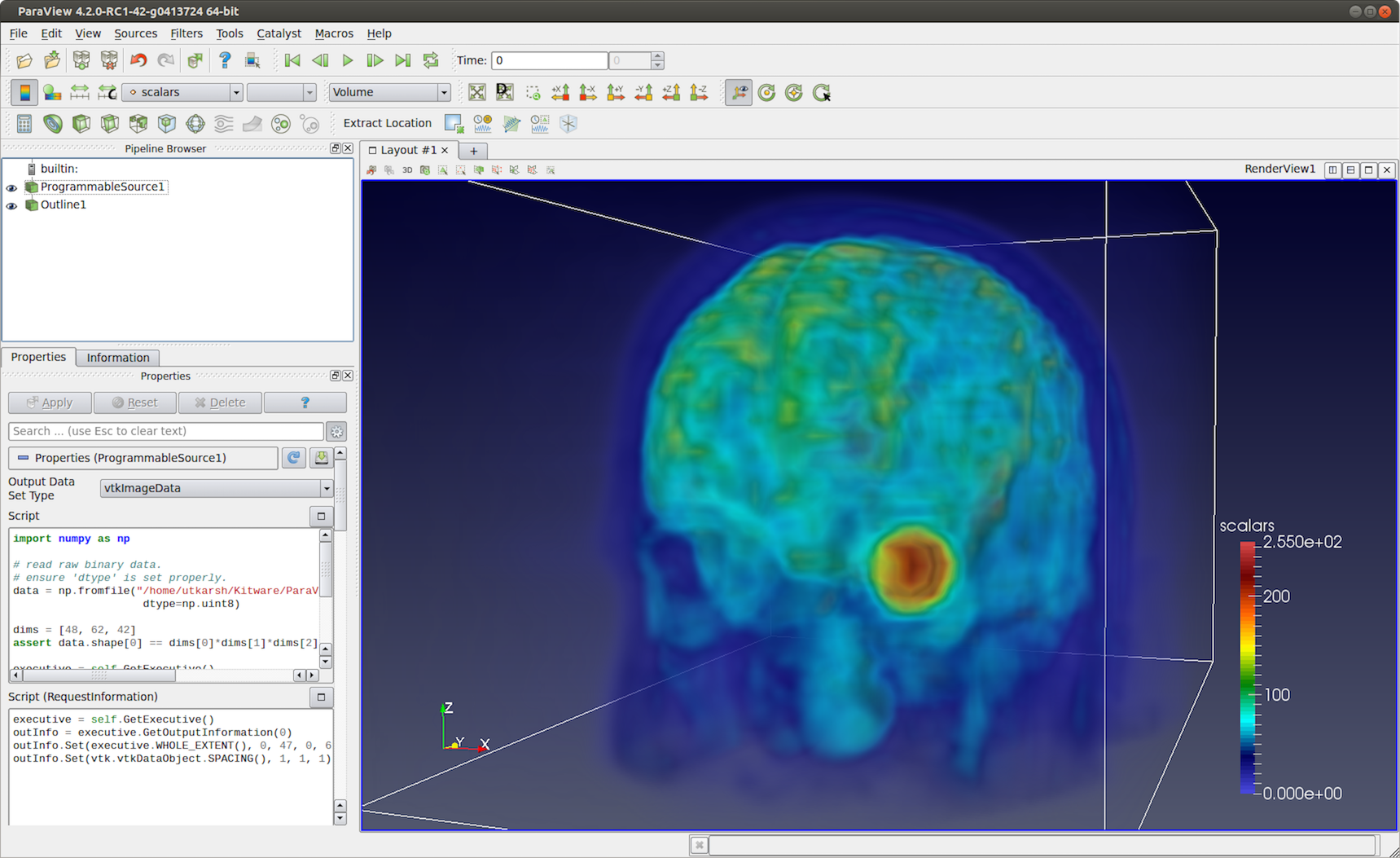
Fig. 4.20 Programmable Source used to read HeadMRVolume.raw file available in the VTK data repository.
4.2.5. Helix source
Here is another polydata source example. This time, we generate the data programmatically.
# Code for 'Script'
#This script generates a helix curve.
#This is intended as the script of a 'Programmable Source'
import math
import numpy as np
from vtk.numpy_interface import algorithms as algs
from vtk.numpy_interface import dataset_adapter as dsa
numPts = 80 # Points along Helix
length = 8.0 # Length of Helix
rounds = 3.0 # Number of times around
# Compute the point coordinates for the helix.
index = np.arange(0, numPts, dtype=np.int32)
scalars = index * rounds * 2 * math.pi / numPts
x = index * length / numPts;
y = np.sin(scalars)
z = np.cos(scalars)
# Create a (x,y,z) coordinates array and associate that with
# points to pass to the output dataset.
coordinates = algs.make_vector(x, y, z)
pts = vtk.vtkPoints()
pts.SetData(dsa.numpyTovtkDataArray(coordinates, 'Points'))
output.SetPoints(pts)
# Add scalars to the output point data.
output.PointData.append(index, 'Index')
output.PointData.append(scalars, 'Scalars')
# Next, we need to define the topology i.e.
# cell information. This helix will be a single
# polyline connecting all the points in order.
ptIds = vtk.vtkIdList()
ptIds.SetNumberOfIds(numPts)
for i in xrange(numPts):
#Add the points to the line. The first value indicates
#the order of the point on the line. The second value
#is a reference to a point in a vtkPoints object. Depends
#on the order that Points were added to vtkPoints object.
#Note that this will not be associated with actual points
#until it is added to a vtkPolyData object which holds a
#vtkPoints object.
ptIds.SetId(i, i)
# Allocate the number of 'cells' that will be added. We are just
# adding one vtkPolyLine 'cell' to the vtkPolyData object.
output.Allocate(1, 1)
# Add the poly line 'cell' to the vtkPolyData object.
output.InsertNextCell(vtk.VTK_POLY_LINE, ptIds)
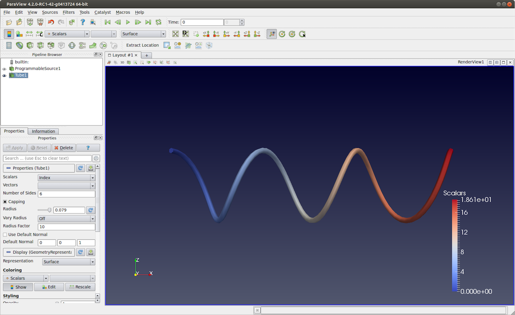
Fig. 4.21 Programmable Source output generated using the script in
Section 4.2.5. This visualization uses Tube
filter to make the output polyline more prominent.
4.3. Recipes for Programmable Filter
One of the differences between the Programmable Source and the
Programmable Filter is that the latter expects at least 1 input. Of course,
the code in the Programmable Filter is free to disregard the input entirely
and work exactly as Programmable Source . Programmable Filter is
designed to customize data transformations. For example, it is useful when you
want to compute derived quantities using expressions not directly possible with
Python Calculator and Calculator or when you want to use other Python
packages or even VTK filters not exposed in ParaView for processing the inputs.
In this section, we look at various recipes for Programmable Filter s.
4.3.1. Adding a new point/cell data array based on an input array
Python Calculator provides an easy mechanism of computing derived
variables. You can also use the Programmable Filter .
Typically, for such cases, ensure that the Output DataSet Type is set to
Same as Input .
# Code for 'Script'
# 'inputs' is set to an array with data objects produced by inputs to
# this filter.
# Get the first input.
input0 = inputs[0]
# compute a value.
dataArray = input0.PointData["V"] / 2.0
# To access cell data, you can use input0.CellData.
# 'output' is a variable set to the output dataset.
output.PointData.append(dataArray, "V_half")
The thing to note about this code is that it will work as expected even when the input dataset is a composite dataset such as a Multiblock dataset ( Section 3.1.10). Refer to Section 5 for details on how this works. There are cases, however, when you may want to explicitly iterate over blocks in an input multiblock dataset. For that, you can use the following snippet.
input0 = inputs[0]
if input0.IsA("vtkCompositeDataSet"):
# iterate over all non-empty blocks in the input
# composite dataset, including multiblock and AMR datasets.
for block in input0:
processBlock(block)
else:
processBlock(input0)
4.3.2. Computing tetrahedra volume
This recipe computes the volume for each tetrahedral cell in the input dataset.
You can always simply use the Python Calculator to compute cell volume
using the expression volume(inputs[0]). This recipe is provided to
illustrate the API.
Ensure that the output type is set to Same as Input , and this filter assumes
the input is an unstructured grid ( Section 3.1.7).
# Code for 'Script'.
import numpy as np
# This filter computes the volume of the tetrahedra in an unstructured mesh.
# Note, this is just an illustration and not the most efficient way for
# computing cell volume. You should use 'Python Calculator' instead.
input0 = inputs[0]
numTets = input0.GetNumberOfCells()
volumeArray = np.empty(numTets, dtype=np.float64)
for i in xrange(numTets):
cell = input0.GetCell(i)
p1 = input0.GetPoint(cell.GetPointId(0))
p2 = input0.GetPoint(cell.GetPointId(1))
p3 = input0.GetPoint(cell.GetPointId(2))
p4 = input0.GetPoint(cell.GetPointId(3))
volumeArray[i] = vtk.vtkTetra.ComputeVolume(p1,p2,p3,p4)
output.CellData.append(volumeArray, "Volume")
4.3.3. Labeling common points between two datasets
In this example, the Programmable Filter takes two input datasets: A and B. It
outputs dataset B with a new scalar array that labels the points in B that
are also in A. You should select two datasets in the pipeline browser and then
apply the programmable filter.
# Code for 'Script'
# Get the two inputs
A = inputs[0]
B = inputs[1]
# use len(inputs) to determine now many inputs are connected
# to this filter.
# We use numpy.in1d to test all which point coordinate components
# in B are present in A as well.
maskX = np.in1d(B.Points[:,0], A.Points[:,0])
maskY = np.in1d(B.Points[:,1], A.Points[:,1])
maskZ = np.in1d(B.Points[:,2], A.Points[:,2])
# Combining each component mask, we get the mask for point
# itself.
mask = maskX & maskY & maskZ
# Now convert it to uint8, since bool arrays
# cannot be passed back to the VTK pipeline.
mask = np.asarray(mask, dtype=np.uint8)
# Initialize the output and add the labels array
# This ShallowCopy is needed since by default the output is
# initialized to be a shallow copy of the first input (inputs[0]),
# but we want it to be a description of the second input.
output.ShallowCopy(B.VTKObject)
output.PointData.append(mask, "labels")
Note in the script above the two inputs are defined in an inputs array. The
order of elements in this array is determined by the order the data sources were
selected in the Pipeline Browser . Hence, inputs[0] is the first data source
selected and inputs[1] is the second.
4.4. Python Algorithm
Programmable Source and Programmable Filter are convenient ways to
prototype a Python-based data processing module. If you want to distribute such
modules, or package them into modules with user interfaces,
for example, then VTKPythonAlgorithmBase -based approach is recommended instead.
Here, you write a Python class by subclassing VTKPythonAlgorithmBase and
implementing methods to do the data processing, just like any other VTK-based
filter or source. Using Python syntactic add-ons called decorators to
annotate your class, you can easily expose the class to ParaView as a filter or
a source, and ParaView will automatically add UI widgets to control parameters, etc.
Let’s start with the simple script featured in
Fig. 4.19. Here’s the Python script to
create a VTKPythonAlgorithmBase subclass for the same operation.
from vtkmodules.vtkCommonDataModel import vtkDataSet
from vtkmodules.util.vtkAlgorithm import VTKPythonAlgorithmBase
from vtkmodules.numpy_interface import dataset_adapter as dsa

class HalfVFilter(VTKPythonAlgorithmBase):
    def __init__(self):
        VTKPythonAlgorithmBase.__init__(self)

    def RequestData(self, request, inInfo, outInfo):
        # get the first input.
        input0 = dsa.WrapDataObject(vtkDataSet.GetData(inInfo[0]))

        # compute a value.
        data = input0.PointData["V"] / 2.0

        # add to output
        output = dsa.WrapDataObject(vtkDataSet.GetData(outInfo))
        output.PointData.append(data, "V_half");
        return 1
To expose this filter in ParaView, you have to add decorators to the class definition as follows:
# same imports as earlier.
from vtkmodules.vtkCommonDataModel import vtkDataSet
from vtkmodules.util.vtkAlgorithm import VTKPythonAlgorithmBase
from vtkmodules.numpy_interface import dataset_adapter as dsa

# new module for ParaView-specific decorators.
from paraview.util.vtkAlgorithm import smproxy, smproperty, smdomain

@smproxy.filter(label="Half-V Filter")
@smproperty.input(name="Input")
class HalfVFilter(VTKPythonAlgorithmBase):
    # the rest of the code here is unchanged.
    def __init__(self):
        VTKPythonAlgorithmBase.__init__(self)

    def RequestData(self, request, inInfo, outInfo):
        # get the first input.
        input0 = dsa.WrapDataObject(vtkDataSet.GetData(inInfo[0]))

        # compute a value.
        data = input0.PointData["V"] / 2.0

        # add to output
        output = dsa.WrapDataObject(vtkDataSet.GetData(outInfo))
        output.PointData.append(data, "V_half");
        return 1
To use this new filter, save this to a *.py file, and load it as a plugin using
the Plugin Manager from Tools > Plugin Manager. On success, you will
see a Half-V Filter in the Filters menu.
Besides exposing class as filters, or sources, you can use the decorators to add UI widgets to call methods on the class to set parameters.
The follow examples adds a new source named Python-based Superquadric Source Example , with UI to control various parameters.
# to add a source, instead of a filter, use the `smproxy.source` decorator.
@smproxy.source(label="Python-based Superquadric Source Example")
class PythonSuperquadricSource(VTKPythonAlgorithmBase):
    """This is dummy VTKPythonAlgorithmBase subclass that
    simply puts out a Superquadric poly data using a vtkSuperquadricSource
    internally"""
    def __init__(self):
        VTKPythonAlgorithmBase.__init__(self,
                nInputPorts=0,
                nOutputPorts=1,
                outputType='vtkPolyData')
        from vtkmodules.vtkFiltersSources import vtkSuperquadricSource
        self._realAlgorithm = vtkSuperquadricSource()

    def RequestData(self, request, inInfo, outInfo):
        from vtkmodules.vtkCommonDataModel import vtkPolyData
        self._realAlgorithm.Update()
        output = vtkPolyData.GetData(outInfo, 0)
        output.ShallowCopy(self._realAlgorithm.GetOutput())
        return 1

    # for anything too complex or not yet supported, you can explicitly
    # provide the XML for the method.
    @smproperty.xml("""
        <DoubleVectorProperty name="Center"
            number_of_elements="3"
            default_values="0 0 0"
            command="SetCenter">
            <DoubleRangeDomain name="range" />
            <Documentation>Set center of the superquadric</Documentation>
        </DoubleVectorProperty>""")
    def SetCenter(self, x, y, z):
        self._realAlgorithm.SetCenter(x,y,z)
        self.Modified()

    # In most cases, one can simply use available decorators.
    @smproperty.doublevector(name="Scale", default_values=[1, 1, 1])
    @smdomain.doublerange()
    def SetScale(self, x, y, z):
        self._realAlgorithm.SetScale(x,y,z)
        self.Modified()

    @smproperty.intvector(name="ThetaResolution", default_values=16)
    def SetThetaResolution(self, x):
        self._realAlgorithm.SetThetaResolution(x)
        self.Modified()

    @smproperty.intvector(name="PhiResolution", default_values=16)
    @smdomain.intrange(min=0, max=1000)
    def SetPhiResolution(self, x):
        self._realAlgorithm.SetPhiResolution(x)
        self.Modified()

    @smproperty.doublevector(name="Thickness", default_values=0.3333)
    @smdomain.doublerange(min=1e-24, max=1.0)
    def SetThickness(self, x):
        self._realAlgorithm.SetThickness(x)
        self.Modified()
On loading this script as a plugin and creating the Python-based Superquadric Source Example
source, the Properties panel will be populated
as shown in Fig. 4.22.
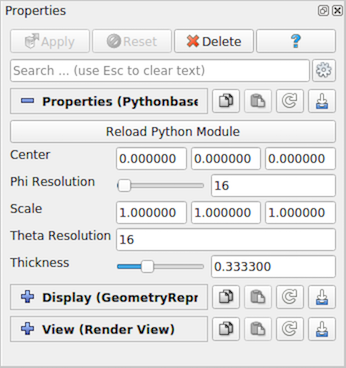
Fig. 4.22 Properties panel automatically generated from a decorated Python
class, PythonSuperquadricSource .
The decorators also enable us to add new readers and writers. Here is an example writer that uses NumPy to write tables as compressed binary arrays.
# `smproxy.writer` decorator register the module as writer for the provided file
# extension.
@smproxy.writer(extensions="npz", file_description="NumPy Compressed Arrays", support_reload=False)
@smproperty.input(name="Input", port_index=0)
# this domain lets ParaView know which types of data this writer can write.
@smdomain.datatype(dataTypes=["vtkTable"], composite_data_supported=False)
class NumpyWriter(VTKPythonAlgorithmBase):
    def __init__(self):
        VTKPythonAlgorithmBase.__init__(self, nInputPorts=1, nOutputPorts=0, inputType='vtkTable')
        self._filename = None

    @smproperty.stringvector(name="FileName", panel_visibility="never")
    @smdomain.filelist()
    def SetFileName(self, fname):
        """Specify filename for the file to write."""
        if self._filename != fname:
            self._filename = fname
            self.Modified()

    def RequestData(self, request, inInfoVec, outInfoVec):
        from vtkmodules.vtkCommonDataModel import vtkTable
        from vtkmodules.numpy_interface import dataset_adapter as dsa

        table = dsa.WrapDataObject(vtkTable.GetData(inInfoVec[0], 0))
        kwargs = {}
        for aname in table.RowData.keys():
            kwargs[aname] = table.RowData[aname]

        import numpy
        numpy.savez_compressed(self._filename, **kwargs)
        return 1

    def Write(self):
        self.Modified()
        self.Update()