6. Remote and parallel visualization

One of the goals of the ParaView application is enabling data analysis and visualization for large datasets. ParaView was born out of the need for visualizating simulation results from simulations run on supercomputing resources that are often too big for a single desktop machine to handle. To enable interactive visualization of such datasets, ParaView uses remote and/or parallel data processing. The basic concept is that if a dataset cannot fit on a desktop machine due to memory or other limitations, we can split the dataset among a cluster of machines, driven from your desktop. In this chapter, we will look at the basics of remote and parallel data processing using ParaView. For information on setting up clusters, please refer to the ParaView Wiki [ThePCommunity].

Did you know?

Remote and parallel processing are often used together, but they refer to different concepts, and it is possible to have one without the other.

In the case of ParaView, remote processing refers to the concept of having a client, typically paraview or pvpython, connecting to a pvserver, which could be running on a different, remote machine. All the data processing and, potentially, the rendering can happen on the pvserver. The client drives the visualization process by building the visualization pipeline and viewing the generated results.

Parallel processing refers to a concept where instead of single core — which we call a rank — processing the entire dataset, we split the dataset among multiple ranks. Typically, an instance of pvserver runs in parallel on more than one rank. If a client is connected to a server that runs in parallel, we are using both remote and parallel processing.

In the case of pvbatch, we have an application that operates in parallel but without a client connection. This is a case of parallel processing without remote processing.

6.1. Understanding remote processing

Let’s consider a simple use-case. Let’s say you have two computers, one located at your office and another in your home. The one at the office is a nicer, beefier machine with larger memory and computing capabilities than the one at home. That being the case, you often run your simulations on the office machine, storing the resulting files on the disk attached to your office machine. When you’re at work, to visualize those results, you simply launch paraview and open the data file(s). Now, what if you need to do the visualization and data analysis from home? You have several options:

• You can copy the data files over to your home machine and then use paraview to visualize them. This is tedious, however, as you not only have to constantly keep copying/updating your files manually, but your machine has poorer performance due to the decreased compute capabilities and memory available on it!

• You can use a desktop sharing system like Remote Desktop or VNC, but those can be flaky depending on your network connection.

Alternatively, you can use ParaView’s remote processing capabilities. The concept is fairly simple. You have two separate processes: pvserver (which runs on your work machine) and a paraview client (which runs on your home machine). They communicate with each other over sockets (over an SHH tunnel, if needed). As far as using paraview in this mode, it’s no different than how we have been using it so far – you create pipelines and then look at the data produced by those pipelines in views and so on. The pipelines themselves, however, are created remotely on the pvserver process. Thus, the pipelines have access to the disks on your work machine. The Open File dialog will in fact browse the file system on your work machine, i.e., the machine on which pvserver is running. Any filters that you create in your visualization pipeline execute on the pvserver.

While all the data processing happens on the pvserver, when it comes to rendering, paraview can be configured to either do the rendering on the server process and deliver only images to the client (remote rendering) or to deliver the geometries to be rendered to the client and let it do the rendering locally (local rendering). When remote rendering, you’ll be using the graphics capabilities on your work machine (the machine running the pvserver). Every time a new rendering needs to be obtained (for example, when pipeline parameters are changed or you interact with the camera, etc.), the pvserver process will re-render a new image and deliver that to the client. When local rendering, the geometries to be rendered are delivered to the client and the client renders those locally. Thus, not all interactions require server-side processing. Only when the visualization pipeline is updated does the server need to deliver updated geometries to the client.

6.2. Remote visualization in paraview

6.2.1. Starting a remote server

To begin using ParaView for remote data processing and visualization, we must first start the server application pvserver on the remote system. To do this, connect to your remote system using a shell and run:

> pvserver

You will see this startup message on the terminal:

Waiting for client...
Connection URL: cs://myhost:11111
Accepting connection(s): myhost:11111

This means that the server has started and is listening for a connection from a client.

6.2.2. Configuring a server connection

To connect to this server with the paraview client, select File > Connect or click the icon in the toolbar to bring up the Choose Server Configuration dialog.

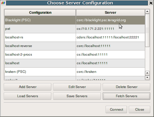
Fig. 6.8 The Choose Server Configuration dialog is used to connect to a server.

Common Errors

If your server is behind a firewall and you are attempting to connect to it from outside the firewall, the connection may not be established successfully. You may also try reverse connections ( Section 6.4) as a workaround for firewalls. Please consult your network manager if you have network connection problems.

Figure Fig. 6.8 shows the Choose Server Configuration dialog with a number of entries for remote servers. In the figure, a number of servers have already been configured, but when you first open this dialog, this list will be empty. Before you can connect to a remote server, you will need to add an entry to the list by clicking on the Add Server button. When you do, you will see the Edit Server Configuration dialog as in Figure Fig. 6.9.

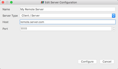
Fig. 6.9 The Edit Server Configuration dialog is used to configure settings for connecting to remote servers.

You will need to set a name for the connection, the server type, the DNS name of the host on which you just started the server, and the port. The default Server Type is set to Client / Server, which means that the server will be listening for an incoming connection from the client. There are several other options for this setting that we will discuss later.

When you are done, click the Configure button. Another dialog, as shown in Fig. 6.10, will appear where you specify how to start the server. Since we started the server manually, we will leave the Startup Type on the default Manual setting. You can optionally set the Startup Type to Command and specify an external shell command to launch a server process.

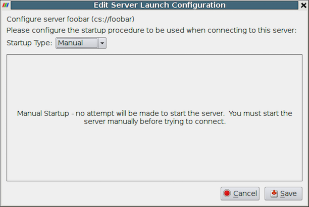
Fig. 6.10 Configure the server manually. It must be started outside of ParaView.

When you click the Save button, this particular server configuration will be saved for future use. You can go back and edit the server configuration by selecting the entry in the list of servers and clicking the Edit Server button in the Choose Server Configuration dialog. You can delete it by clicking the Delete button.

Server configurations can be imported and exported through the Choose Server Configuration dialog. Use the Load Servers button to load a server configuration file and the Save Servers button to save a server configuration file. Files can be exchanged with others to access the same remote servers.

Did you know?

Visualization centers can provide system-wide server configurations on web servers to allow non-experts to simply select an already configured ParaView server. The format of the XML file for saving the server configurations is discussed online on the ParaView Wiki at http://paraview.org/Wiki/Server_Configuration. These site-wide settings can be loaded with the Fetch Servers button.

6.2.3. Connect to the remote server

To connect to the server, select the server configuration you just set up from the configuration list and click Connect . We are now ready to build the visualization pipelines.

Common Errors

ParaView does not perform any kind of authentication when clients attempt to connect to a server. For that reason, we recommend that you do not run pvserver on a computing resource that is open to the outside world.

ParaView also does not encrypt data sent between the client and server. If your data is sensitive, please ensure that proper network security measures have been taken. The typical approach is to use an SSH tunnel.

6.2.4. Managing multiple clients

pvserver can be configured to accept connections from multiple clients at the same time. In this case only one, called the master, can interact with the pipeline. Others clients are only allowed to visualize the data. The Collaboration Panel shares information between connected clients.

To enable this mode, pvserver must be started with the --multi-clients flag:

pvserver --multi-clients

If your remote server is accessible from many users, you may want to restrict the access. This can be done with a connect id. If your client does not have the same connect-id as the server you want to connect to, you will be prompted for a connect-id. Then, if you are the master, you can change the connect-id in the Collaboration Panel .

Note that initial value for connect-id can be set by starting the pvserver (and respectively paraview) with the --connect-id flag, for instance:

pvserver --connect-id=147

The master client can also disable further connections in the Collaboration Panel so you can work alone, for instance. Once you are ready, you may allow other people to connect to the pvserver to share a visualization. This is the default feature when pvserver is started with --multi-clients --disable-further-connections.

6.2.5. Setting up a client/server visualization pipeline

Using paraview when connected to a remote server is not any different than when it’s being used in the default stand-alone mode. The only difference, as far as the user interface goes, is that the Pipeline Browser reflects the name of the server to which you are connected. The address of the server connection next to the icon changes from builtin to cs://myhost:11111 .

Since the data processing pipelines are executing on the server side, all file I/O also happens on the server side. Hence, the Open File dialog, when opening a new data file, will browse the file system local to the pvserver executable and not the paraview client.

6.3. Remote visualization in pvpython

The pvpython executable can be used by itself for visualization of local data, but it can also act as a client that connects to a remote pvserver. Before creating a pipeline in pvpython, use the Connect function:

# Connect to remote server "myhost" on the default port, 11111
>>> Connect("myhost") # Connect to remote server "myhost" on a
                      # specified port
>>> Connect("myhost", 11111)

Now, when new sources are created, the data produced by the sources will reside on the server. In the case of pvpython, all data remains on the server and images are generated on the server too. Images are sent to the client for display or for saving to the local filesystem.

6.4. Reverse connections

It is frequently the case that remote computing resources are located behind a network firewall, making it difficult to connect a client outside the firewall to a server behind it. ParaView provides a way to set up a reverse connection that reverses the usual client server roles when establishing a connection.

To use a remote connection, two steps must be performed. First, in paraview, a new connection must be configured with the connection type set to reverse. To do this, open the Choose Server Configuration dialog through the File > Connect menu item. Add a new connection, setting the Name to myhost (reverse)'', and select ``Client / Server (reverse connection) for Server Type . Click Configure . In the Edit Server Launch Configuration dialog that comes up, set the Startup Type to Manual . Save the configuration. Next, select this configuration and click Connect . A message window will appear showing that the client is awaiting a connection from the server.

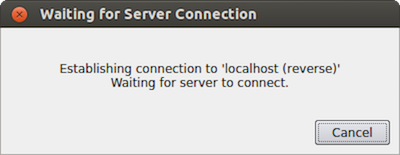
Fig. 6.11 Message window showing that the client is awaiting a connection from a server.

Second, pvserver must be started with the --reverse-connection (-rc) flag. To tell pvserver the name of the client, set the --client-host (-ch) command-line argument to the hostname of the machine on which the paraview client is running. You can specify a port with the --server-port (-sp) command-line argument.

pvserver -rc --client-host=mylocalhost --server-port=11111

When the server starts, it prints a message indicating the success or failure of connecting to the client. When the connection is successful, you will see the following text in the shell:

Connecting to client (reverse connection requested)...
Connection URL: csrc://mylocalhost:11111
Client connected.

To wait for reverse connections from a pvserver in pvpython, you use ReverseConnect instead of Connect .

# To wait for connections from a 'pvserver' on the default port 11111
>>> ReverseConnect()

# Optionally, you can specify the port number as the argument.
>>> ReverseConnect(11111)

6.5. Understanding parallel processing

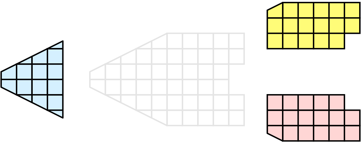
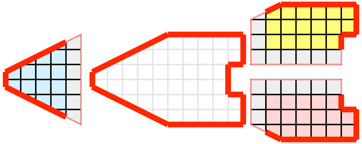
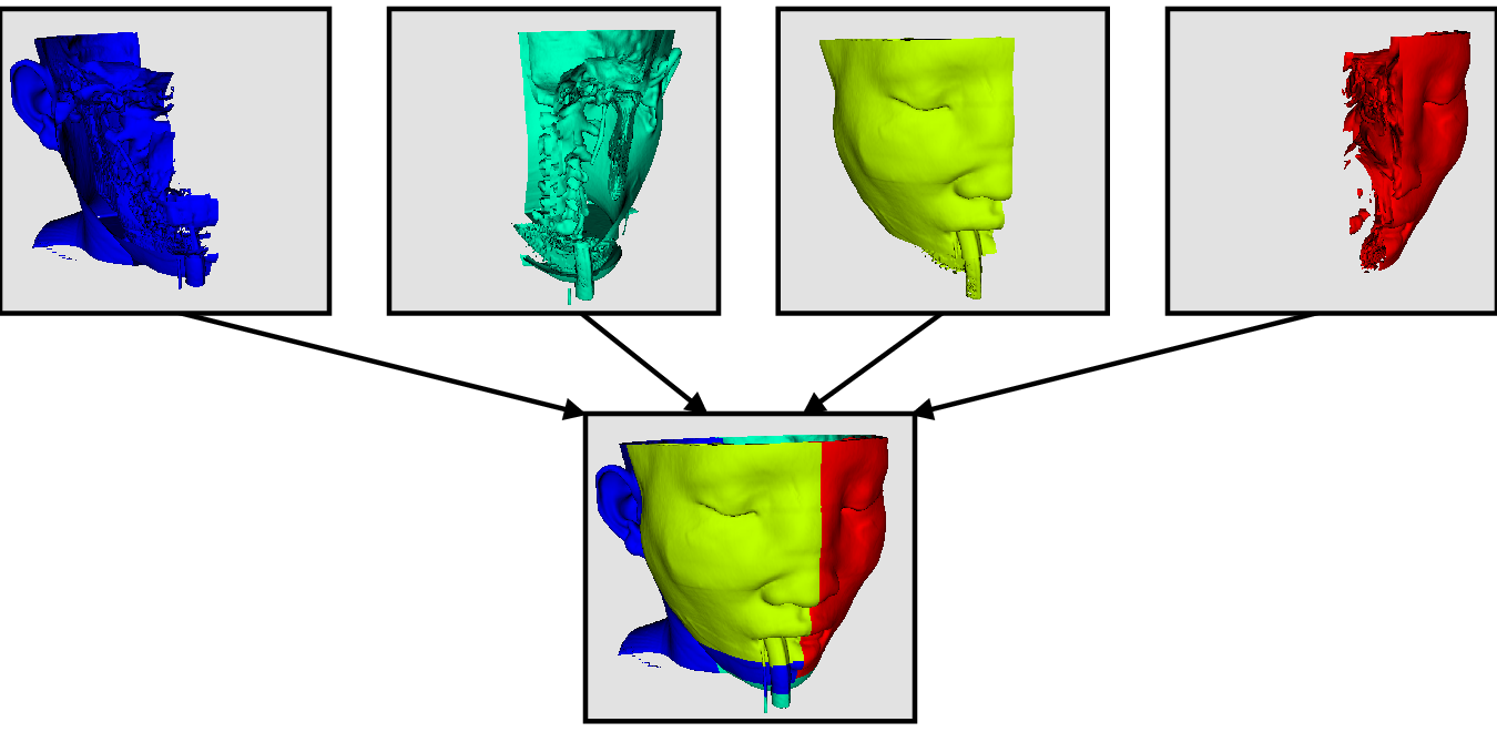
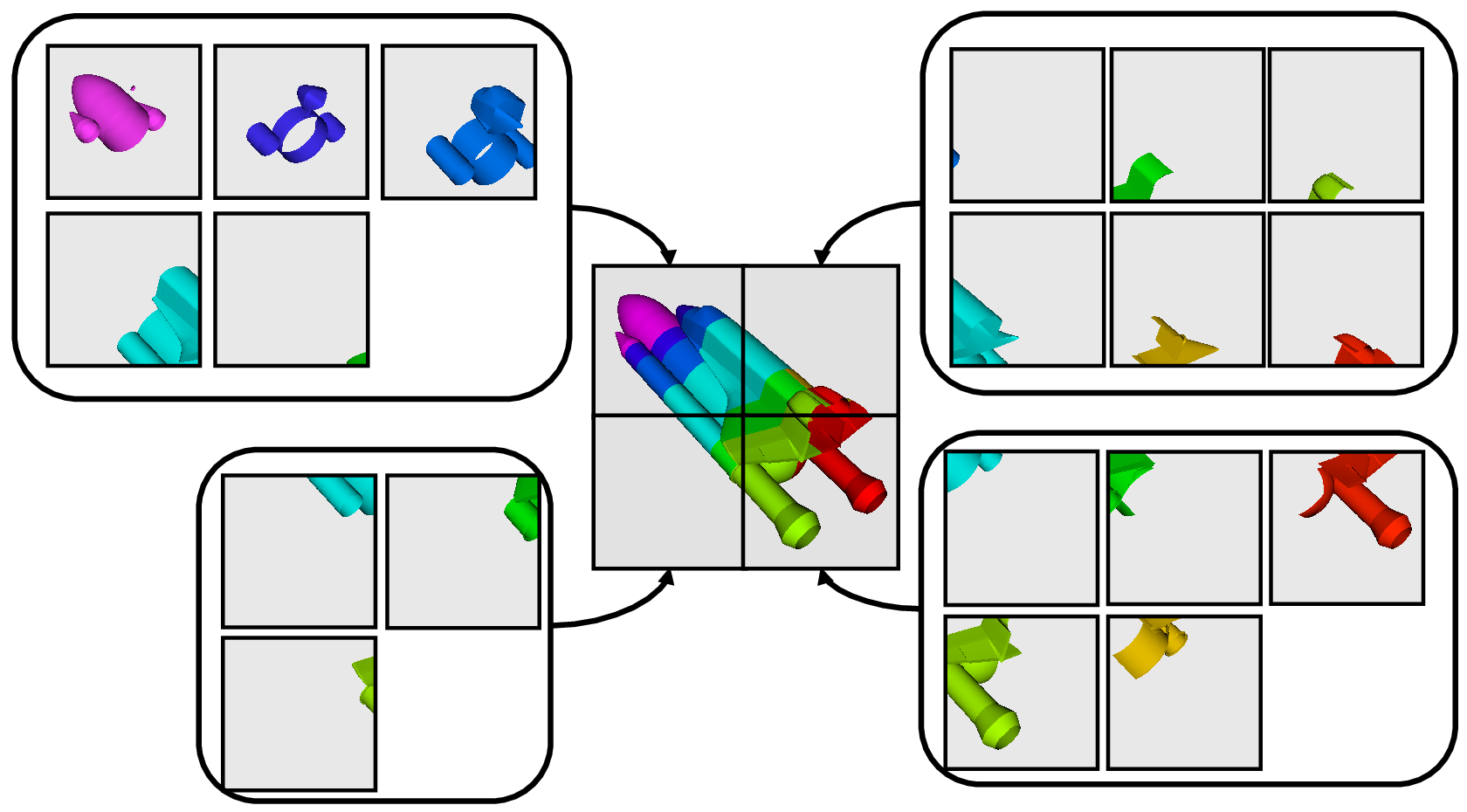
Parallel processing, put simply, implies processing the data in parallel, simultaneously using multiple workers. Typically, these workers are different processes that could be running on a multicore machine or on several nodes of a cluster. Let’s call these ranks. In most data processing and visualization algorithms, work is directly related to the amount of data that needs to be processed, i.e., the number of cells or points in the dataset. Thus, a straight-forward way of distributing the work among ranks is to split an input dataset into multiple chunks and then have each rank operate only an independent set of chunks. Conveniently, for most algorithms, the result obtained by splitting the dataset and processing it separately is same as the result that we’d get if we processed the dataset in a single chunk. There are, of course, exceptions. Let’s try to understand this better with an example. For demonstration purposes, consider this very simplified mesh.

Now, let us say we want to perform visualizations on this mesh using three processes. We can divide the cells of the mesh as shown below with the blue, yellow, and pink regions.

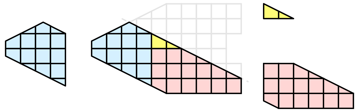
Once partitioned, some visualization algorithms will work by simply allowing each process to independently run the algorithm on its local collection of cells. Take clipping as an example. Let’s say that we define a clipping plane and give that same plane to each of the processes.

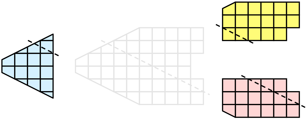
Each process can independently clip its cells with this plane. The end result is the same as if we had done the clipping serially. If we were to bring the cells together (which we would never actually do for large data for obvious reasons), we would see that the clipping operation took place correctly.

6.5.1. Ghost levels

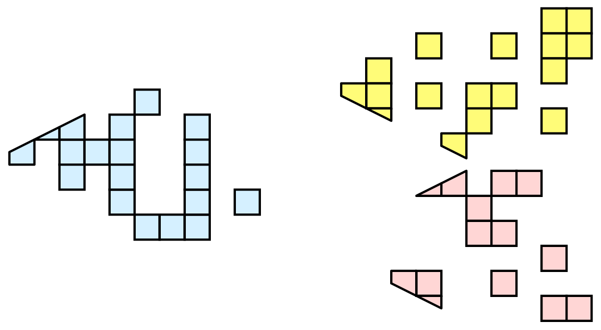
Unfortunately, blindly running visualization algorithms on partitions of cells does not always result in the correct answer. As a simple example, consider the external faces algorithm. The external faces algorithm finds all cell faces that belong to only one cell, thereby, identifying the boundaries of the mesh.

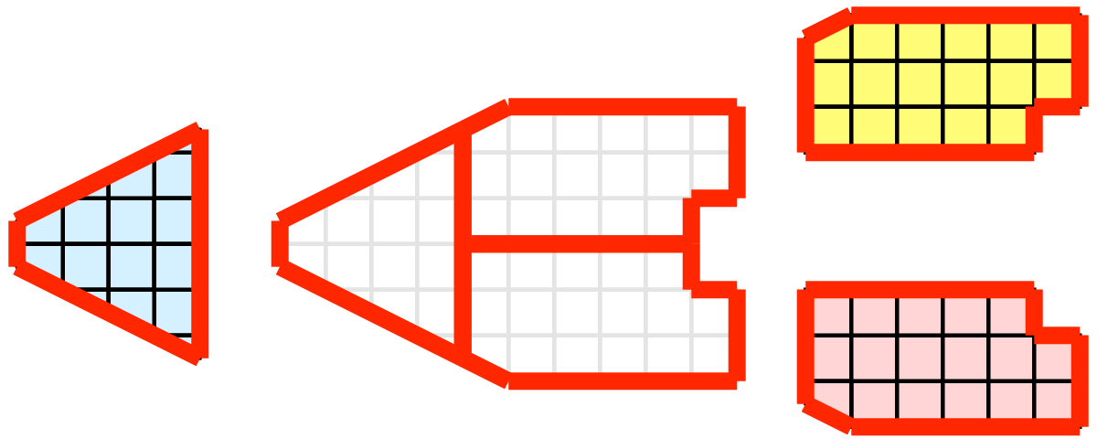
Oops! We see that when all the processes ran the external faces algorithm independently, many internal faces where incorrectly identified as being external. This happens where a cell in one partition has a neighbor in another partition. A process has no access to cells in other partitions, so there is no way of knowing that these neighboring cells exist.

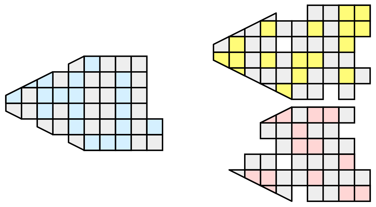
The solution employed by ParaView and other parallel visualization systems is to use ghost cells . Ghost cells are cells that are held in one process but actually belong to another. To use ghost cells, we first have to identify all the neighboring cells in each partition. We then copy these neighboring cells to the partition and mark them as ghost cells, as indicated with the gray colored cells in the following example.

When we run the external faces algorithm with the ghost cells, we see that we are still incorrectly identifying some internal faces as external. However, all of these misclassified faces are on ghost cells, and the faces inherit the ghost status of the cell from which it came. ParaView then strips off the ghost faces, and we are left with the correct answer.

In this example, we have shown one layer of ghost cells: only those cells that are direct neighbors of the partition’s cells. ParaView also has the ability to retrieve multiple layers of ghost cells, where each layer contains the neighbors of the previous layer not already contained in a lower ghost layer or in the original data itself. This is useful when we have cascading filters that each require their own layer of ghost cells. They each request an additional layer of ghost cells from upstream, and then remove a layer from the data before sending it downstream.

6.5.2. Data partitioning

Since we are breaking up and distributing our data, it is prudent to address the ramifications of how we partition the data. The data shown in the previous example has a spatially coherent partitioning. That is, all the cells of each partition are located in a compact region of space. There are other ways to partition data. For example, you could have a random partitioning.

Random partitioning has some nice features. It is easy to create and is friendly to load balancing. However, a serious problem exists with respect to ghost cells.

In this example, we see that a single level of ghost cells nearly replicates the entire dataset on all processes. We have thus removed any advantage we had with parallel processing. Because ghost cells are used so frequently, random partitioning is not used in ParaView.

6.5.3. D3 Filter

The previous section described the importance of load balancing and ghost levels for parallel visualization. This section describes how to achieve that.

Load balancing and ghost cells are handled automatically by ParaView when you are reading structured data (image data, rectilinear grid, and structured grid). The implicit topology makes it easy to break the data into spatially coherent chunks and identify where neighboring cells are located.

It is an entirely different matter when you are reading in unstructured data (poly data and unstructured grid). There is no implicit topology and no neighborhood information available. ParaView is at the mercy of how the data was written to disk. Thus, when you read in unstructured data, there is no guarantee of how well-load balanced your data will be. It is also unlikely that the data will have ghost cells available, which means that the output of some filters may be incorrect.

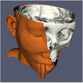
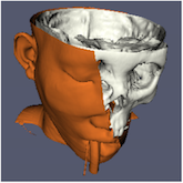
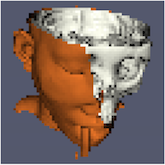
Fortunately, ParaView has a filter that will both balance your unstructured data and create ghost cells. This filter is called D3, which is short for distributed data decomposition. Using D3 is easy; simply attach the filter (located in Filters > Alphabetical > D3) to whatever data you wish to repartition.

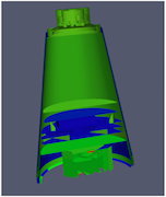
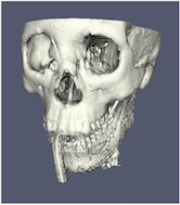
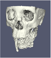
The most common use case for D3 is to attach it directly to your unstructured grid reader. Regardless of how well-load balanced the incoming data might be, it is important to be able to retrieve ghost cell so that subsequent filters will generate the correct data. The example above shows a cutaway of the extract surface filter on an unstructured grid. On the left, we see that there are many faces improperly extracted because we are missing ghost cells. On the right, the problem is fixed by first using the D3 filter.

6.6. Ghost Cells Generator

If your unstructured grid data is already partitioned satisfactorily but does not have ghost cells, it is possible to generate them using the Ghost Cells Generator filter. This filter can be attached to a source just like the D3 filter. Unlike D3 , it will not repartition the dataset, it will only generate ghost cells, which is needed for some algorithms to execute correctly.

The Ghost Cells Generator has several options. Build If Required tells the filter to generate ghost cells only if required by a downstream filter. Since computing ghost cells is a computationally and communications intensive process, turning this option on can potentially save a lot of processing time. The Minimum Number Of Ghost Levels specifies at least how many ghost levels should be generated if Build If Required is off. Downstream filters may request more ghost levels than this minimum, in which case the Ghost Cells Generator will generate the requested number of ghost levels. The Use Global Ids option makes use of a GlobalIds array if it is present if on. If off, ghost cells are determined by coincident points.

6.7. ParaView architecture

Before we see how to use ParaView for parallel data processing, let’s take a closer look at the ParaView architecture. ParaView is designed as a three-tier client-server architecture. The three logical units of ParaView are as follows.

• Data Server The unit responsible for data reading, filtering, and writing. All of the pipeline objects seen in the pipeline browser are contained in the data server. The data server can be parallel.

• Render Server The unit responsible for rendering. The render server can also be parallel, in which case built-in parallel rendering is also enabled.

• Client The unit responsible for establishing visualization. The client controls the object creation, execution, and destruction in the servers, but does not contain any of the data (thus allowing the servers to scale without bottlenecking on the client). If there is a GUI, that is also in the client. The client is always a serial application.

These logical units need not by physically separated. Logical units are often embedded in the same application, removing the need for any communication between them. There are three modes in which you can run ParaView.

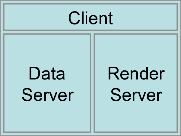
The first mode, with which you are already familiar, is standalone mode. In standalone mode, the client, data server, and render server are all combined into a single serial application. When you run the paraview application, you are automatically connected to a builtin server so that you are ready to use the full features of ParaView.

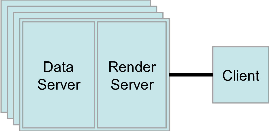
The second mode is client-server mode. In client-server mode, you execute the pvserver program on a parallel machine and connect to it with the paraview client application (or pvpython). The pvserver program has both the data server and render server embedded in it, so both data processing and rendering take place there. The client and server are connected via a socket, which is assumed to be a relatively slow mode of communication, so data transfer over this socket is minimized. We saw this mode of operation in Section 6.2.

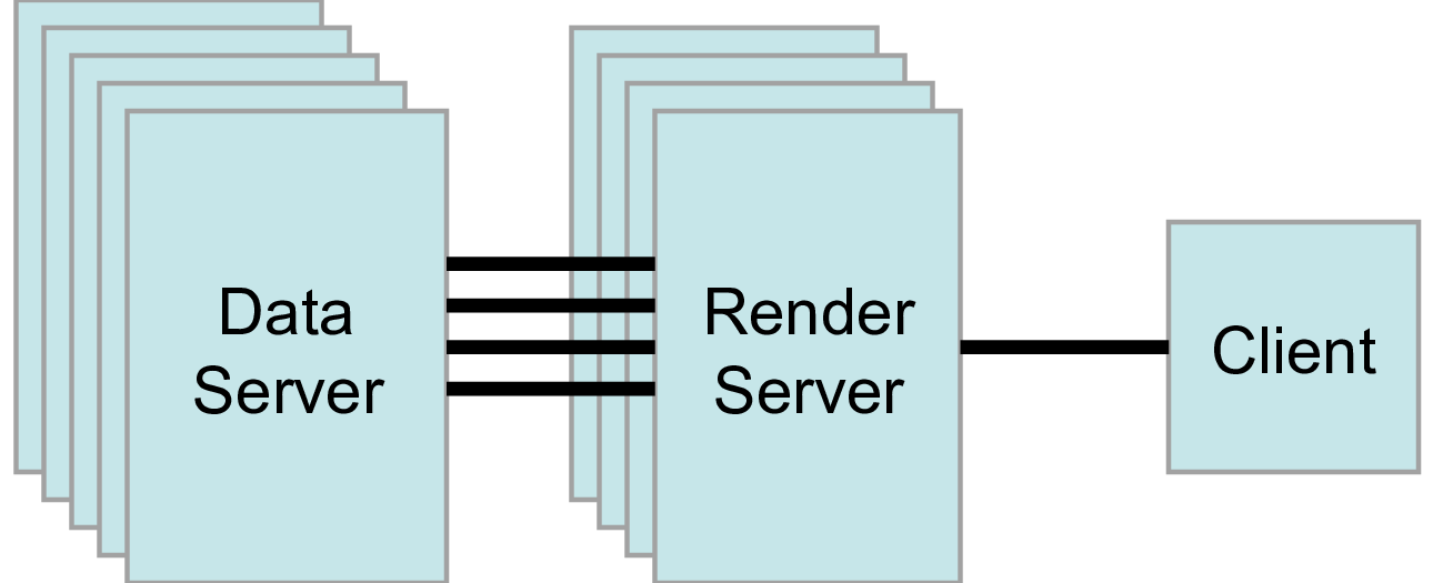
The third mode is client-render server-data server mode. In this mode, all three logical units are running in separate programs. As before, the client is connected to the render server via a single socket connection. The render server and data server are connected by many socket connections, one for each process in the render server. Data transfer over the sockets is minimized.

Although the client-render server-data server mode is supported, we almost never recommend using it. The original intention of this mode is to take advantage of heterogeneous environments where one might have a large, powerful computational platform and a second smaller parallel machine with graphics hardware in it. However, in practice, we find any benefit is almost always outstripped by the time it takes to move geometry from the data server to the render server. If the computational platform is much bigger than the graphics cluster, then use software rendering on the large computational platform. If the two platforms are about the same size, just perform all the computation on the graphics cluster. The executables used for this mode are paraview (or pvpython) (acting as the client), pvdataserver for the data-server, and pvrenderserver for the render-server.

6.8. Parallel processing in paraview and pvpython

To leverage parallel processing capabilities in paraview or pvpython, one has to use remote visualization, i.e., one has to connect to a pvserver. The processing for connecting to this pvserver is not different from what we say in Section 6.2 and Section 6.3. The only thing that changes is how the pvserver is launched.

You can start pvserver to run on more than one processing core using mpirun .

mpirun -np 4 pvserver

This will run pvserver on four processing cores. It will still listen for an incoming connection from a client on the default port. The big difference when running pvserver this way is that when data is loaded from a source, it will be distributed across the four cores if the data source is parallel aware and supports distributing the data across the different processing cores.

To see how this data is distributed, run pvserver as the command above and connect to it with paraview. Next, create another Sphere source using Source > Sphere. Change the array to color by to vtkProcessId . You will see an image like Figure Fig. 6.12.

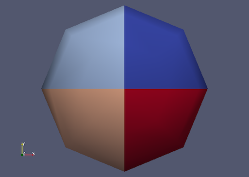
Fig. 6.12 Sphere source colored by vtkProcessId array that encodes the processing core on which the sphere data resides. Here, the sphere data is split among the four processing cores invoked by the command mpirun -np 4 pvserver.

If a data reader or source is not parallel aware, you can still get the benefits of spreading the data among processing cores by using the D3 filter. This filter partitions a dataset into convex regions and transfers each region to a different processing core. To see an example of how D3 partitions a dataset, create a Source > Wavelet while paraview is still connected to the pvserver. Next, select Filters > Alphabetical > D3 and click Apply . The output of D3 will not initially appear different from the original wavelet source. If you color by vtkProcessId , however, you will see the four partitions that have been distributed to the server processing cores.

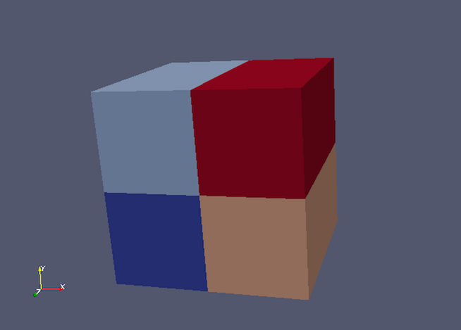
Fig. 6.13 Wavelet source processed by the D3 filter and colored by vtkProcessId array. Note how four regions of the image data are split evenly among the four processing cores when pvserver is run with mpirun -np 4 pvserver .

6.9. Using pvbatch

In Section 6.8, we said that to use parallel processing capabilities, one has to use remote visualization, i.e., one must use ParaView in a client-server mode with the client (paraview or pvpython) connecting to a server (pvserver) that is being run in parallel using mpirun . However, there is one exception: pvbatch. pvpython and pvbatch are quite similar in that both are similar to the python

executable that can be used to run Python scripts. The extra thing that these executables do when compared with the standard python is that they initialize the environment so that any scripts that you run will be able to locate the ParaView Python modules and libraries automatically. pvpython is exactly like the paraview executable without the GUI. You can think of it as the GUI from paraview is replaced by a Python interpreter in pvpython. pvbatch, on the other hand, can be thought of a pvserver where, instead of taking the control command from a remote client (paraview or pvpython), in pvbatch, the commands are taken from a Python script that is executed in the pvbatch executable itself. Since pvbatch is akin to the pvserver, unlike pvpython, it can be run in parallel using mpirun . In that case, the root rank (or the first rank or the rank with index $0$) is the one that acts as the client, interpreting the Python script to execute the commands. Since pvbatch is designed to act is its own server, you cannot connect to a remote server in the Python script, i.e., you cannot use simple.Connect . Furthermore, pvbatch is designed for batch operation, which means that you can only specify the Python script as a command line argument. Unlike pvpython, you cannot run this executable to get an interactive shell to enter Python commands.

# process the sample.py script in single process mode.
> pvbatch sample.py

# process the sample.py script in parallel.
> mpirun -np 4 sample.py

In general, you should use pvpython if you will be using the interpreter interactively and pvbatch if you are running in parallel.

6.10. Fetching data to the client

Section 3.3 describes how to obtain information about a data object, but not how to access the data object itself. This section describes several ways to access data from within a Python script. The client/server nature of ParaView requires a couple steps to access the raw data. The Python script runs on the client side in either pvpython or paraview, so one step involves moving the data from the server to the client. This can be accomplished with the following:

from paraview.simple import *
Connect("myhost")

# Create a sphere source on myhost
s = Sphere()
full_sphere = servermanager.Fetch(s)

Here, the full dataset is moved from the server to the client.

The second step is required to deal with the fact that data on the remote server may be split across distributed processes. By default, servermanager.Fetch(s) appends all the pieces on the different remote processes and produces the appended data set on the client. The exact append operation depends on the type of dataset being retrieved. Composite datasets are merged by treating the dataset piece on each distributed process as a block merged into a new multiblock dataset, polygonal datasets are appended into a single polygonal dataset, rectilinear grids are appended into a single rectilinear grid, and other datasets are appended into an unstructured grid. Distributed image datasets cannot currently be fetched to the client. Care must be taken when fetching an entire dataset to the client because the data that fits on many distributed processes on a remote system may not fit in client memory.

Another option is to fetch just a single piece of the dataset on one remote process to the client. To do this, pass the rank number of the remote process from which you want to retrieve the data to the Fetch function, e.g.,

# Retrieve the piece of the data set on remote process 2
s = Sphere()
sphere_piece = servermanager.Fetch(s, 2)

Lastly, servermanager.Fetch provides a way to apply helper filters to the dataset that run at two stages. The filter for the first stage is applied to the data on each remote process, and the filter for the second stage is applied to the results from the first stage after they are gathered to the root server process. The results from the second stage of filtering are then transferred from the root server process to the client.

In the next example, the Extract Surface filter is applied to a source with data on each process in the first stage. The results are then assembled with the Append Geometry filter and sent to the client.

s = Sphere()
extract = servermanager.filters.ExtractSurface()
append = servermanager.filters.AppendGeometry()
full_surface = servermanager.Fetch(s, extract, append)

The second filter must be able to accept multiple connections and handle the output dataset type from the first filter.

6.11. Rendering

Rendering is the process of synthesizing the images that you see based on your data. The ability to effectively interact with your data depends highly on the speed of the rendering. Thanks to advances in 3D hardware acceleration, fueled by the computer gaming market, we have the ability to render 3D quickly even on moderately-priced computers. But, of course, the speed of rendering is proportional to the amount of data being rendered. As data gets bigger, the rendering process naturally gets slower.

To ensure that your visualization session remains interactive, ParaView supports two modes of rendering that are automatically flipped as necessary. In the first mode, still render , the data is rendered at the highest level of detail. This rendering mode ensures that all of the data is represented accurately. In the second mode, interactive render , speed takes precedence over accuracy. This rendering mode endeavors to provide a quick rendering rate regardless of data size.

While you are interacting with a 3D view (for example, rotating, panning, or zooming with the mouse), ParaView uses an interactive render. This is because, during the interaction, a high frame rate is necessary to make these features usable and because each frame is immediately replaced with a new rendering while the interaction is occurring so that fine details are less important during this mode. At any time when interaction of the 3D view is not taking place, ParaView uses a still render so that the full detail of the data is available as you study it. As you drag your mouse in a 3D view to move the data, you may see an approximate rendering. The full detail will be presented as soon as you release the mouse button.

The interactive render is a compromise between speed and accuracy. As such, many of the rendering parameters concern when and how lower levels of detail are used.

6.11.1. Basic Rendering Settings

Some of the most important rendering options are the LOD parameters. During interactive rendering, the geometry may be replaced with a lower level of detail ( LOD ), an approximate geometry with fewer polygons.

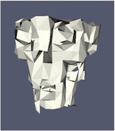
The resolution of the geometric approximation can be controlled. In the proceeding images, the left image is the full resolution, the middle image is the default decimation for interactive rendering, and the right image is ParaView’s maximum decimation setting.

The 3D rendering parameters are located in the settings dialog box, which is accessed in the menu from the Edit > Settings menu (ParaView > Preferences on the Mac). The rendering options in the dialog are in the Render View tab.

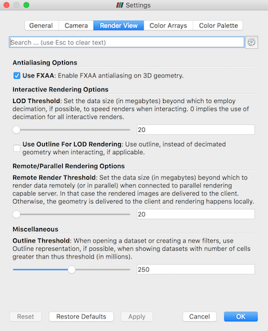
The options pertaining to the geometric decimation for interactive rendering are located in a section labeled Interactive Rendering Options . Some of these options are considered advanced, so to access them, you have to either toggle on the advanced options with the button or search for the option using the edit box at the top of the dialog. The interactive rendering options include the following.

• LOD Threshold : Set the data size at which to use a decimated geometry in interactive rendering. If the geometry size is under this threshold, ParaView always renders the full geometry. Increase this value if you have a decent graphics card that can handle larger data. Try decreasing this value if your interactive renders are too slow.

• LOD Resolution : Set the factor that controls how large the decimated geometry should be. This control is set to a value between 0 and 1. 0 produces a very small number of triangles but, possibly, with a lot of distortion. 1 produces more detailed surfaces but with larger geometry.

• Non Interactive Render Delay : Add a delay between an interactive render and a still render. ParaView usually performs a still render immediately after an interactive motion is finished (for example, releasing the mouse button after a rotation). This option can add a delay that can give you time to start a second interaction before the still render starts, which is helpful if the still render takes a long time to complete.

• Use Outline For LOD Rendering : Use an outline in place of decimated geometry. The outline is an alternative for when the geometry decimation takes too long or still produces too much geometry. However, it is more difficult to interact with just an outline.

ParaView contains many more rendering settings. Here is a summary of some other settings that can effect the rendering performance regardless of whether ParaView is run in client-server mode or not. These options are spread among several categories, and several are considered advanced.

• Translucent Rendering Options

  • Depth Peeling : Enable or disable depth peeling. Depth peeling is a technique ParaView uses to properly render translucent surfaces. With it, the top surface is rendered and then “peeled away” so that the next lower surface can be rendered and so on. If you find that making surfaces transparent really slows things down or renders completely incorrectly, then your graphics hardware may not be implementing the depth peeling extensions well; try shutting off depth peeling.

  • Depth Peeling for Volumes : Include volumes in depth peeling to correctly intermix volumes and translucent polygons.

  • Maximum Number Of Peels : Set the maximum number of peels to use with depth peeling. Using more peels allows more depth complexity, but allowing less peels runs faster. You can try adjusting this parameter if translucent geometry renders too slow or translucent images do not look correct.

• Miscellaneous

  • Outline Threshold : When creating very large datasets, default to the outline representation. Surface representations usually require ParaView to extract geometry of the surface, which takes time and memory. For data with sizes above this threshold, use the outline representation, which has very little overhead, by default instead.

  • Show Annotation : Show or hide annotation providing rendering performance information. This information is handy when diagnosing performance problems.

Note that this is not a complete list of ParaView rendering settings. We have left out settings that do not significantly affect rendering performance. We have also left out settings that are only valid for parallel client-server rendering, which are discussed in Section 6.11.4.

6.11.2. Basic Parallel Rendering

When performing parallel visualization, we are careful to ensure that the data remains partitioned among all of the processes up to and including the rendering processes. ParaView uses a parallel rendering library called IceT . IceT uses a sort-last algorithm for parallel rendering. This parallel rendering algorithm has each process independently render its partition of the geometry and then composites the partial images together to form the final image.

The preceding diagram is an oversimplification. IceT contains multiple parallel image compositing algorithms such as binary tree , binary swap , and radix-k that efficiently divide work among processes using multiple phases.

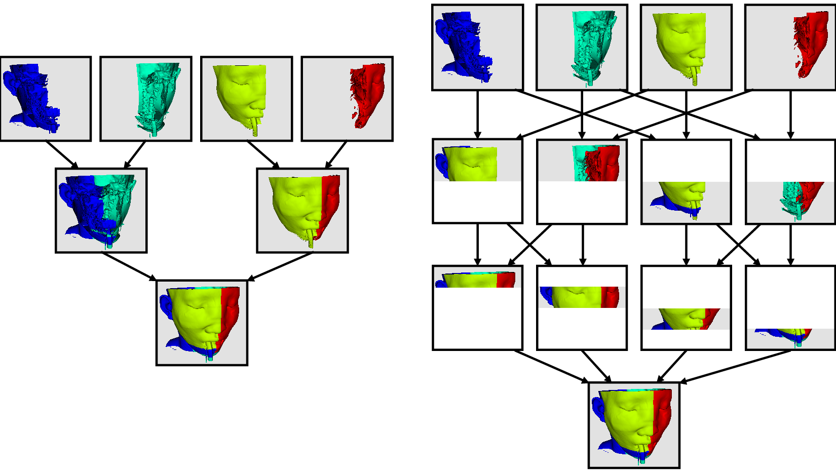
The wonderful thing about sort-last parallel rendering is that its efficiency is completely insensitive to the amount of data being rendered. This makes it a very scalable algorithm and well suited to large data. However, the parallel rendering overhead does increase linearly with the number of pixels in the image. Consequently, some of the rendering parameters deal with the image size.

IceT also has the ability to drive tiled displays, which are large, high-resolution displays comprising an array of monitors or projectors. Using a sort-last algorithm on a tiled display is a bit counterintuitive because the number of pixels to composite is so large. However, IceT is designed to take advantage of spatial locality in the data on each process to drastically reduce the amount of compositing necessary. This spatial locality can be enforced by applying the Filters > Alphabetical > D3 filter to your data.

Because there is an overhead associated with parallel rendering, ParaView has the ability to turn off parallel rendering at any time. When parallel rendering is turned off, the geometry is shipped to the location where display occurs. Obviously, this should only happen when the data being rendered is small.

6.11.3. Image Level of Detail

The overhead incurred by the parallel rendering algorithms is proportional to the size of the images being generated. Also, images generated on a server must be transfered to the client, a cost that is also proportional to the image size. To help increase the frame rate during interaction, ParaView introduces a new LOD parameter that controls the size of the images.

During interaction while parallel rendering, ParaView can optionally subsample the image. That is, ParaView will reduce the resolution of the image in each dimension by a factor during interaction. Reduced images will be rendered, composited, and transfered. On the client, the image is inflated to the size of the available space in the GUI.

The resolution of the reduced images is controlled by the factor with which the dimensions are divided. In the proceeding images, the left image has the full resolution. The following images were rendered with the resolution reduced by a factor of 2, 4, and 8, respectively.

ParaView also has the ability to compress images before transferring them from server to client. Compression, of course, reduces the amount of data transferred and, therefore, makes the most of the available bandwidth. However, the time it takes to compress and decompress the images adds to the latency.

ParaView contains several different image compression algorithms for client-server rendering. The first uses LZ4 compression that is designed for high-speed compression and decompression. The second option is a custom algorithm called Squirt , which stands for Sequential Unified Image Run Transfer. Squirt is a run-length encoding compression that reduces color depth to increase run lengths. The third algorithm uses the Zlib compression library, which implements a variation of the Lempel-Ziv algorithm. Zlib typically provides better compression than Squirt, but it takes longer to perform and, hence, adds to the latency. paraview Windows and Linux executables include a compression option that uses NVIDIA’s NVPipe library for hardware-accelerated compression and decompression if a Kepler-class or higher NVIDIA GPU is available.

6.11.4. Parallel Render Parameters

Like the other 3D rendering parameters, the parallel rendering parameters are located in the Settings dialog. The parallel rendering options in the dialog are in the Render View tab (intermixed with several other rendering options such as those described in Section 6.11.1). The parallel and client-server options are divided among several categories, and several are considered advanced.

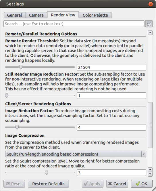
• Remote/Parallel Rendering Options

  • Remote Render Threshold : Set the data size at which to render remotely in parallel or to render locally. If the geometry is over this threshold (and ParaView is connected to a remote server), the data is rendered in parallel remotely, and images are sent back to the client. If the geometry is under this threshold, the geometry is sent back to the client, and images are rendered locally on the client.

  • Still Render Image Reduction Factor : Set the sub-sampling factor for still (non-interactive) rendering. Some large displays have more resolution than is really necessary, so this sub-sampling reduces the resolution of all images displayed.

• Client/Server Rendering Options

  • Image Reduction Factor : Set the interactive subsampling factor. The overhead of parallel rendering is proportional to the size of the images generated. Thus, you can speed up interactive rendering by specifying an image subsampling rate. When this box is checked, interactive renders will create smaller images, which are then magnified when displayed. This parameter is only used during interactive renders.

• Image Compression

  • Before images are shipped from server to client, they can optionally be compressed using one of three available compression algorithms: LZ4 , Squirt , or Zlib . To make the compression more effective, either algorithm can reduce the color resolution of the image before compression. The sliders determine the amount of color bits saved. Full color resolution is always used during a still render.

  • Suggested image compression presets are provided for several common network types. When attempting to select the best image compression options, try starting with the presets that best match your connection.

6.11.5. Parameters for Large Data

The default rendering parameters are suitable for most users. However, when dealing with very large data, it can help to tweak the rendering parameters. While the optimal parameters depend on your data and the hardware on which ParaView is running, here are several pieces of advice that you should follow.

• If there is a long pause before the first interactive render of a particular dataset, it might be the creation of the decimated geometry. Try using an outline instead of decimated geometry for interaction. You could also try lowering the factor of the decimation to 0 to create smaller geometry.

• Avoid shipping large geometry back to the client. The remote rendering will use the power of the entire server to render and ship images to the client. If remote rendering is off, geometry is shipped back to the client. When you have large data, it is always faster to ship images than to ship data. (Although, if your network has a high latency, this could become problematic for interactive frame rates.)

• Adjust the interactive image sub-sampling for client-server rendering as needed. If image compositing is slow, if the connection between client and server has low bandwidth, or if you are rendering very large images, then a higher subsample rate can greatly improve your interactive rendering performance.

• Make sure Image Compression is on. It has a tremendous effect on desktop delivery performance, and the artifacts it introduces, which are only there during interactive rendering, are minimal. Lower bandwidth connections can try using Zlib instead of Squirt compression. Zlib will create smaller images at the cost of longer compression/decompression times.

• If the network connection has a high latency, adjust the parameters to avoid remote rendering during interaction. In this case, you can try turning up the remote rendering threshold a bit, and this is a place where using the outline for interactive rendering is effective.

• If the still (non-interactive) render is slow, try turning on the delay between interactive and still rendering to avoid unnecessary renders.