3. Comparative visualization
Comparative visualization in ParaView refers to the ability to create
side-by-side visualizations for comparing with one another. In its most
basic form, you can indeed use ParaView’s ability to show multiple views side by
side to set up simultaneous visualizations. But, that can get cumbersome too
quickly. Let’s take a look at a simple example: Let’s say you want to do a parameter
study where you want to compare isosurfaces generated by a set of isovalues in a
dataset. To set up such a visualization, you’ll need to first create as many
Render View s as isovalues. Then, create just as many Contour filters,
setting each one up with a right isovalue for the contour to generate and
display the result in one of the views. As the number of isovalues increases,
you can see how this can get tedious. It is highly error prone, as you need to
keep track of which view shows which isovalue. Now, imagine after having set up
the entire visualization that you need to change the Representation type for
all the of the isosurfaces to Wireframe !
Comparative View s were designed to handle such use-cases. Instead of
creating separate views, you create a single view Render View
(Comparative) . The view itself comprises of a configurable
\(m\times n\) Render View s. Any data that you show in this view gets shown in
all the internal views simultaneously. Any display property changes, such as
scalar coloring and representation type are also maintained consistently between
these internal views. The interactions in the internal views are linked, so when
you interact with one, all other views update as well. While this is all
nice and well, the real power of Comparative View s becomes apparent
when you set up a parameter to vary across the views. This parameter can be
any of the properties on the pipeline modules such as filter properties and
opacity, or it could be the data time. Each of these internal views will
now render the result obtained by setting the parameter as per your selection.
Going back to our original example, we will create a single Contour filter
that we show in Render View (Comparative) with as many internal views as
the isovalue to compare. Next, we will set up a parameter study for varying the
Isosurfaces property on the Contour filter, and, viola! The view will
generate the comparative visualization for us!
In this chapter, we look at how to configure this view and how to set these
parameters to compare. We limit our discussion to Render View
(Comparative) . However, the same principles are applicable to other comparative
views, including Bar Chart View (Comparative) and Line Chart View
(Comparative) .
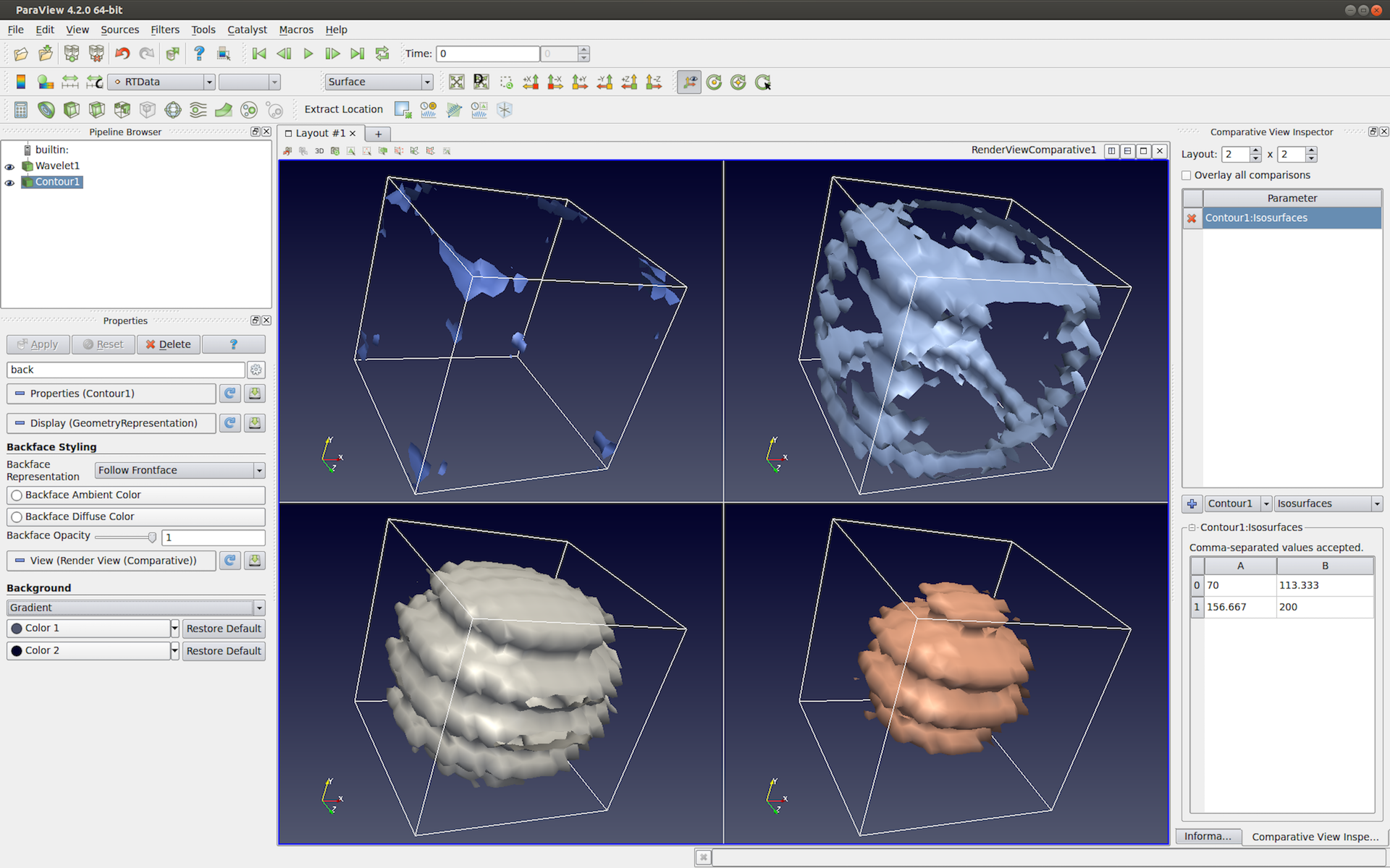
Fig. 3.17 Render View (Comparative) in paraview showing a
parameter study. In this case, we are comparing the visualization generated
using different isovalues for the Contour filter. The Comparative View
Inspector dockpanel (on the right) is used to configure the parameter study.
3.1. Setting up a comparative view
To create Render View (Comparative) in paraview, split or
close the active view and select Render View (Comparative) from the new
view creation widget. paraview will immediately show four Render View s
laid out in a \(2\times 2\) grid. While you cannot resize these internal views,
notice that you can still split the view frame and create other views if
needed.
The Properties panel will show properties similar to those available on the
Render View under the View properties section. If you change any of
these properties, they will affect all these internal views, e.g., setting the
Background color to Gradient will make all the views show a gradient
background.
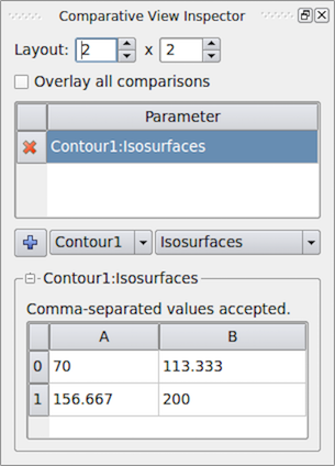
Fig. 3.18 Comparative View Inspector in paraview used to configure the active comparative view.
To configure the comparative view itself, you must to use the
Comparative View Inspector ( Fig. 3.18)
accessible from the View menu. The
Comparative View Inspector is a dockable panel that is enabled when the
active view is a comparative view.
To change how many internal views are used in the active comparative view and
how they are laid out, use the Layout . The first value is the number of
views in the horizontal direction and the second is the count in the vertical
direction.
Besides doing a parameter study in side-by-side views, you can also show all the
results in a single view. For that, simply check the
Overlay all comparisons checkbox. When checked, instead of getting a grid of \(m\times n\)
views, you will only see one view with all visible data displayed \(m\times n\)
times.
To show data in this view is the same as any other view: Make this view active and
use the Pipeline Browser to toggle the eyeball icons to show data produced
by the selected pipeline module(s). Showing any dataset in this view will
result in the data being shown in all the internal views simultaneously. As is true with
View properties, with Display properties, changing
Coloring , Styling , or any other properties will reflect in all
internal views.
Since the cameras among the internal views are automatically linked, if you interact with one of the views, all views will also update simultaneously when you release the mouse button.
3.2. Setting up a parameter study
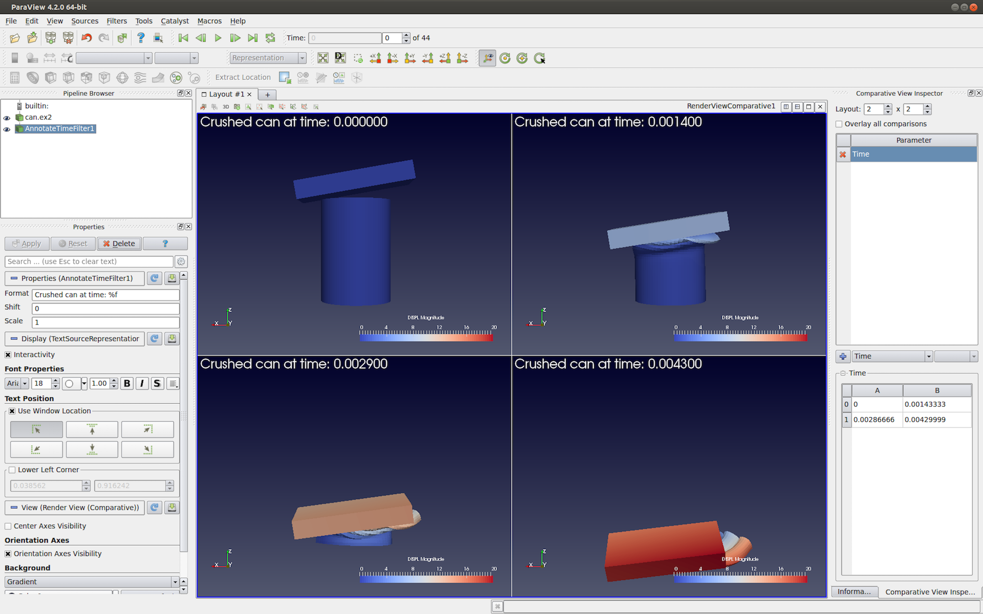
Fig. 3.19 Render View (Comparative) with Annotate Time filter showing
the time for each of the views. In this case, the parameter study is varying
Time across the views.
To understand how to setup a parameter study, let’s go back to our original
example. Our visualization pipeline is simply
Wavelet \(\rightarrow\) Contour (assuming default property values), and we
are showing the result from the Contour filter in the \(2 \times 2\) Render View
(Comparative) with Overlay all comparisons unchecked.
Now, we want to vary the Isosurfaces property value for the visualization
in each of the internal views. That’s our parameter to study. Since that’s a
property on the Contour filter, we select the Contour filter instance.
Then, its property Isosurfaces is in the parameter selection
combo-boxes. To add the parameter to the study, you must hit the
 button.
The parameter Contour1:Isosurfaces will then show up in the Parameter list above the combo-boxes. You can delete this parameter by using the
 button next to the parameter name.
Did you know?
Notice how this mechanism for setting up a parameter study is similar to how animations are set up. In fact, under the cover, the two mechanisms are not that different, and they share a lot of implementation code.
Simultaneously, the table widget below the combo-boxes is populated with a
default set of values for the Isosurfaces . This is where you specify the
parameter values for each of the views. The location of the views matches the
location in the table. Hence, \(0-A\) is the top-left view, \(0-B\) is the second
view from the left in the topmost row, and so on. The parameter value at a
specific location in the table is the value used to generate the visualization
in the corresponding view.
To change the parameter (in our case Isosurfaces ) value, you can double
click on the cell in the table and change it one at a time. Also, to make it
easier to fill the cells with a range of values, you can click and drag over
multiple cells. When you release the mouse, a dialog will prompt you to enter
the data value range ( Fig. 3.20).
In case you selected a combination of rows and columns,
the dialog will also let you select in which direction the parameter is varied
using the range specified. You can choose to vary the parameter horizontally
first, vertically first, or only along one of the directions while keeping the
other constant. This is useful when doing a study with multiple parameters.
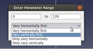
Fig. 3.20 Dialog used to select a range of parameter values and control how to vary them in paraview.
As soon as you change the parameter values, the view will update to reflect the change.
3.3. Adding annotations
You add annotations like color legends, text, and cube-axes
exactly as you would with a regular Render View . As with other
properties, annotations will show up in all of the internal views.
Did you know?
You can use the Annotate Time source or filter to show the data time or
the view time in each of the internal views. If Time is one of the
parameters in your study, the text will reflect the time values for each of
the individual views, as expected ( Fig. 3.19)!