1. Introduction
ParaView is an open-source application for visualizing two- and three-dimensional data sets. The size of the data sets ParaView can handle varies widely depending on the architecture on which the application is run. The platforms supported by ParaView range from single-processor workstations to multiple-processor distributed-memory supercomputers or workstation clusters. Using a parallel machine, ParaView can process very large data sets in parallel and later collect the results. To date, ParaView has been demonstrated to process billions of unstructured cells and to process over a trillion structured cells. ParaView’s parallel framework has run on over 100,000 processing cores.
ParaView’s design contains many conceptual features that make it stand apart from other scientific visualization solutions.
An open-source, scalable, multi-platform visualization application.
Support for distributed computation models to process large data sets.
An open, flexible, and intuitive user interface.
An extensible, modular architecture based on open standards.
A flexible BSD 3-clause license.
Commercial maintenance and support.


ParaView is used by many academic, government, and commercial institutions all over the world. ParaView’s open license makes it impossible to track exactly how many users ParaView has, but it is thought to be many thousands large based on indirect evidence. For example, ParaView is downloaded roughly 100,000 times every year. ParaView also won the HPCwire Readers’ Choice Award in 2010 and 2012 and HPCwire Editors’ Choice Award in 2010 for Best HPC Visualization Product or Technology.
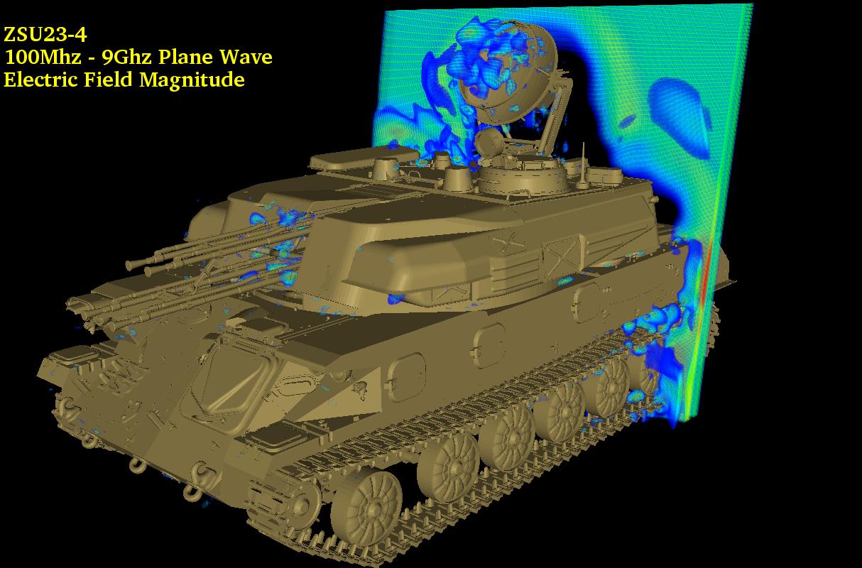
Fig. 1.10 ZSU23-4 Russian Anti-Aircraft vehicle being hit by a planar wave. Image courtesy of Jerry Clarke, US Army Research Laboratory.
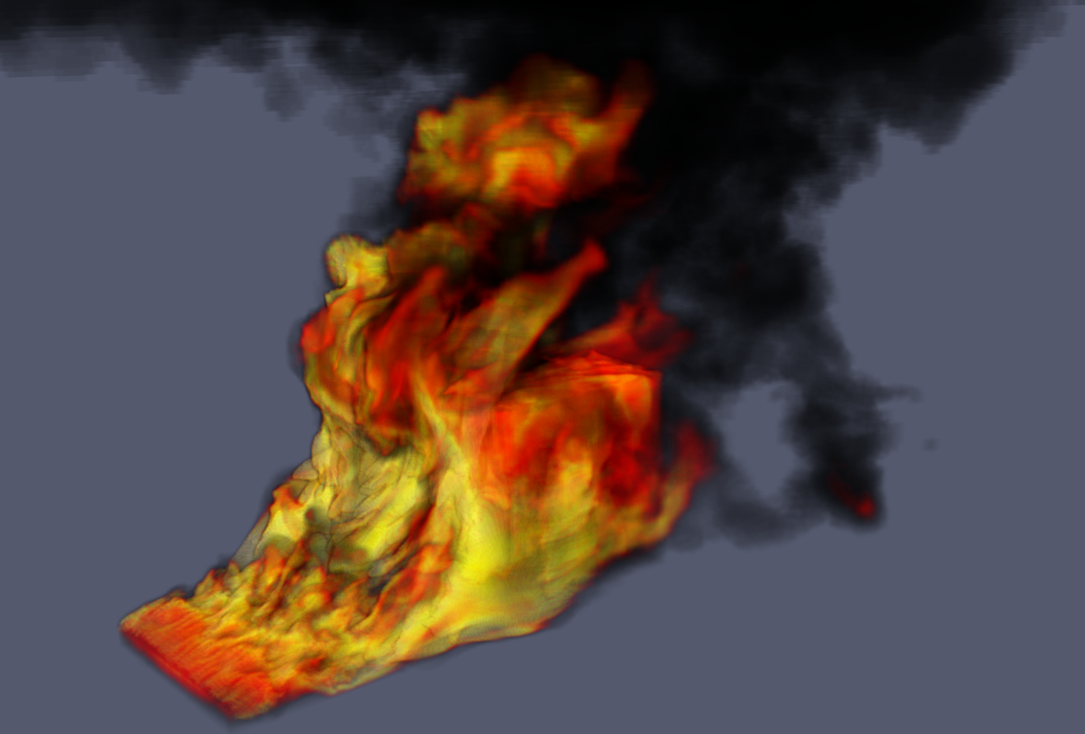
Fig. 1.11 A loosely coupled SIERRA-Fuego-Syrinx-Calore simulation with 10 million unstructured hexahedra cells of objects-in-crosswind fire.
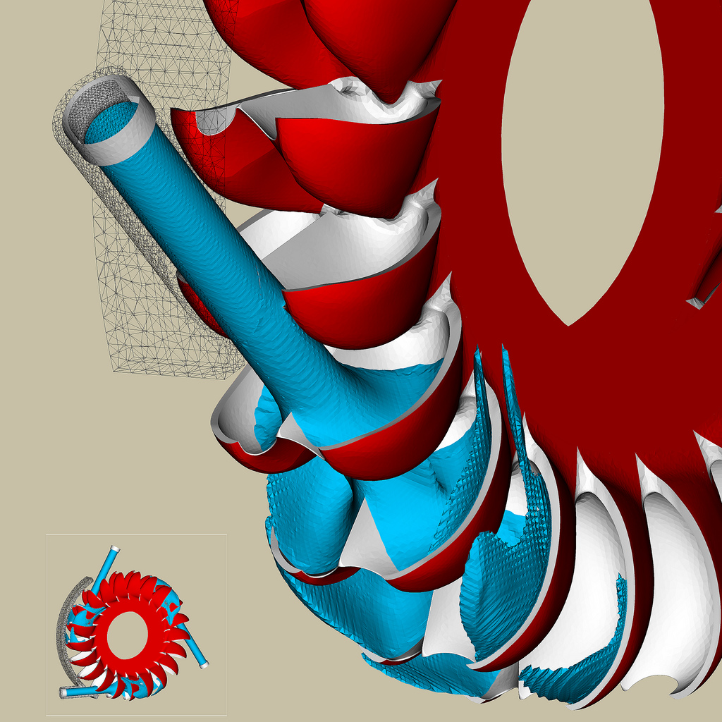
Fig. 1.12 Simulation of a Pelton turbine. Image courtesy of the Swiss National Supercomputing Centre.
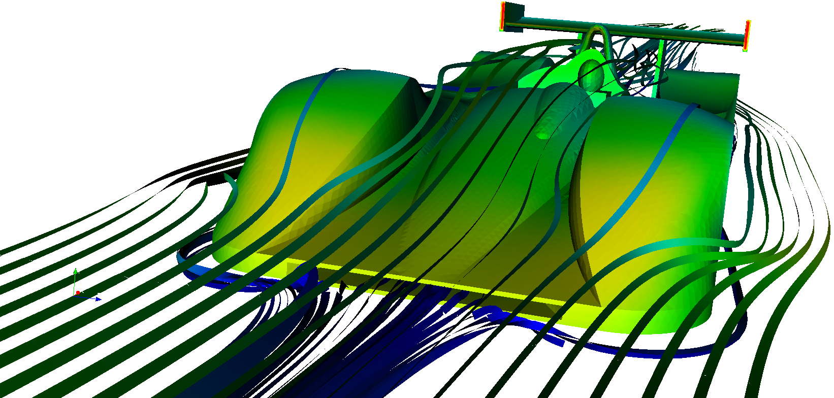
Fig. 1.13 Airflow around a Le Mans Race car. Image courtesy of Renato N. Elias, NACAD/COPPE/UFRJ, Rio de Janerio, Brazil.
As demonstrated in these visualizations, ParaView is a general-purpose tool with a wide breadth of applications. In addition to scaling from small to large data, ParaView provides many general-purpose visualization algorithms as well as some specific to particular scientific disciplines. Furthermore, the ParaView system can be extended with custom visualization algorithms.
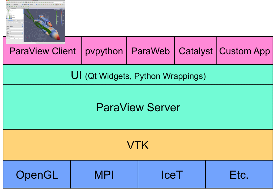
The application most people associate with ParaView is really just a small client application built on top of a tall stack of libraries that provide ParaView with its functionality. Because the vast majority of ParaView features are implemented in libraries, it is possible to completely replace the ParaView GUI with your own custom application. Furthermore, ParaView comes with a application that allows you to automate the visualization and post-processing with Python scripting.
Available to each ParaView application is a library of user interface components to maximize code sharing between them. A library provides the abstraction layer necessary for running parallel, interactive visualization. It relieves the client application from most of the issues concerning if and how ParaView is running in parallel. The Visualization Toolkit (VTK) provides the basic visualization and rendering algorithms. VTK incorporates several other libraries to provide basic functionalities such as rendering, parallel processing, file I/O, and parallel rendering. Although this tutorial demonstrates using ParaView through the ParaView client application, be aware that the modular design of ParaView allows for a great deal of flexibility and customization.
1.1. Development and Funding
The ParaView project started in 2000 as a collaborative effort between Kitware Inc. and Los Alamos National Laboratory. The initial funding was provided by a three year contract with the US Department of Energy ASCI Views program. The first public release, ParaView 0.6, was announced in October 2002. Development of ParaView continued through collaboration of Kitware Inc. with Sandia National Laboratories, Los Alamos National Laboratories, the Army Research Laboratory, and various other academic and government institutions.
In September 2005, Kitware, Sandia National Labs and CSimSoft started the development of ParaView 3.0. This was a major effort focused on rewriting the user interface to be more user friendly and on developing a quantitative analysis framework. ParaView 3.0 was released in May 2007.
Since this time, ParaView development continues. ParaView 4.0 was released in June 2013 and introduced more cohesive GUI controls and better multiblock interaction. Subsequent releases also include the Catalyst library for in situ integration into simulation and other applications. ParaView 5.0 was released in January 2016 and provided a major update to the rendering system. The new rendering takes advantage of OpenGL 3.2 features to provide huge performance improvements. Subsequent releases also added support for ray cast rendering with the OSPRay library.
Development of ParaView continues today. Sandia National Laboratories continues to fund ParaView development through the ASC project. ParaView is part of the SciDAC Scalable Data Management, Analysis, and Visualization (SDAV) Institute Toolkit https://sdav-scidac.org. The US Department of Energy also funds ParaView through Los Alamos National Laboratories and various SBIR projects and other contracts. The US National Science Foundation also often funds ParaView through SBIR projects. Other institutions also have ParaView support contracts: Electricity de France, Mirarco, and oil industry customers. Also, because ParaView is an open source project, other institutions such as the Swiss National Supercomputing Centre contribute back their own development.
1.2. Basics of Visualization
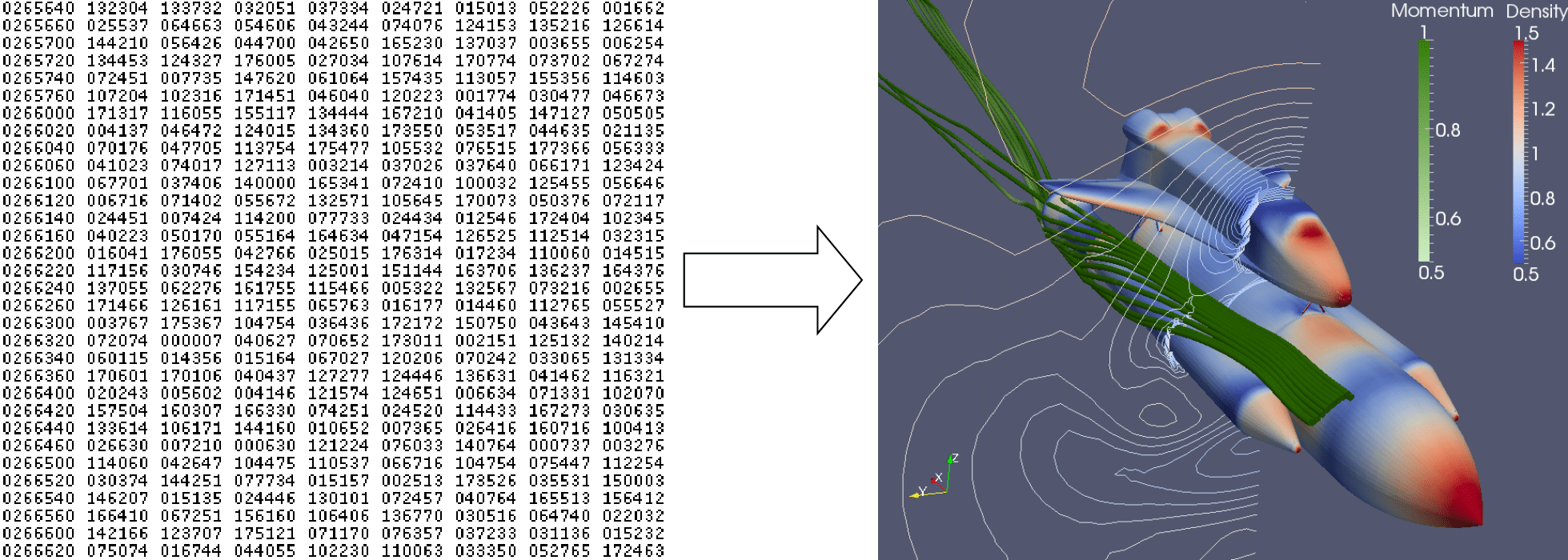
Put simply, the process of visualization is taking raw data and converting it to a form that is viewable and understandable to humans. This allows us to get a better cognitive understanding of our data. Scientific visualization is specifically concerned with the type of data that has a well defined representation in 2D or 3D space. Data that comes from simulation meshes and scanner data is well suited for this type of analysis.
There are three basic steps to visualizing your data: reading, filtering, and rendering. First, your data must be read into ParaView. Next, you may apply any number of filters that process the data to generate, extract, or derive features from the data. Finally, a viewable image is rendered from the data.
ParaView was designed primarily to handle data with spatial representation. Thus the primary data types used in ParaView are meshes.
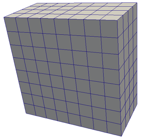
Uniform Rectilinear (Image Data)
A uniform rectilinear grid is a one- two- or three- dimensional array of data. The points are orthonormal to each other and are spaced regularly along each direction.
Non-uniform Rectilinear (Rectilinear Grid)
Similar to the uniform rectilinear grid except that the spacing between points may vary along each axis.
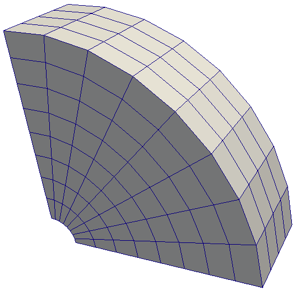
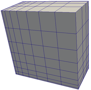
Curvilinear (Structured Grid)
Curvilinear grids have the same topology as rectilinear grids. However, each point in a curvilinear grid can be placed at an arbitrary coordinate (provided that it does not result in cells that overlap or self intersect). Curvilinear grids provide the more compact memory footprint and implicit topology of the rectilinear grids, but also allow for much more variation in the shape of the mesh.
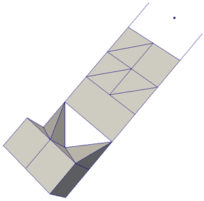
Polygonal (Poly Data)
Polygonal data sets are composed of points, lines, and 2D polygons. Connections between cells can be arbitrary or non-existent. Polygonal data represents the basic rendering primitives. Any data must be converted to polygonal data before being rendered (unless volume rendering is employed), although ParaView will automatically make this conversion.
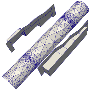
Unstructured Grid
Unstructured data sets are composed of points, lines, 2D polygons, 3D tetrahedra, and nonlinear cells. They are similar to polygonal data except that they can also represent 3D tetrahedra and nonlinear cells, which cannot be directly rendered.
In addition to these basic data types, ParaView also supports multiblock data. A basic multi-block data set is created whenever data sets are grouped together or whenever a file containing multiple blocks is read. ParaView also has some special data types for representing Hierarchical Adaptive Mesh Refinement (AMR), Hierarchical Uniform AMR, Octree, Tabular, and Graph type data sets.
1.3. More Information
There are many places to find more information about ParaView. The manual, titled The ParaView Guide, is available for purchase as a hard copy or can be downloaded for free from https://docs.paraview.org/.
The ParaView web page, https://www.paraview.org/, is also an excellent place to find more information about ParaView. From there you can find helpful links to the ParaView Discourse forum, Wiki pages, and frequently asked questions as well as information about professional support services.
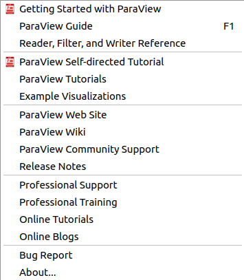
ParaView’s menu is a good place to start to find useful information and contains many links to documentation and training materials. The menu has entries that directly bring up the aforementioned ParaView Guide and web pages. The menu also provides several training materials including a quick Getting Started with ParaView guide, multiple tutorials (including this one), and some example visualizations.