Visualization can be characterized as a process of transforming raw data
produced from experiments or simulations until it takes a form in which it can be
interpreted and analysed. The visualization pipeline introduced in
Section 1.2 formalizes this concept as a data flow
paradigm where a pipeline is set up of sources, filters, and sinks
(collectively called pipeline modules or algorithms). Data flows
through this pipeline, being transformed at each node until it is in a form where
it can be consumed by the sinks. In previous chapters, we saw how to ingest data
into ParaView (Section 2) and how to display it in
views (Section 4). If the data ingested into ParaView
already has all the relevant attribute data, and it is in the form that can be directly
represented in one the existing views, then that is all you would need.
The true power of the visualization process, however, comes from leveraging the
various visualization techniques such as slicing, contouring, clipping, etc.,
which are available as filters. In this chapter, we look at constructing
pipelines to transform data using such filters.
In ParaView, filters are pipeline modules or algorithms that have inputs and
outputs. They take in data on their inputs and produce transformed data or
results on their outputs. A filter can have multiple input and output ports.
The number of input and output ports on a filter is fixed. Each input port accepts
input data for a specific purpose or role within the filter. (E.g., the
ResampleWithDataset filter has two input ports. The one called Input
is the input port through which the dataset providing the attributes to
interpolate is ingested. The other, called Source , is the input port
through which the dataset used as the mesh on which to re-sample is accepted.)
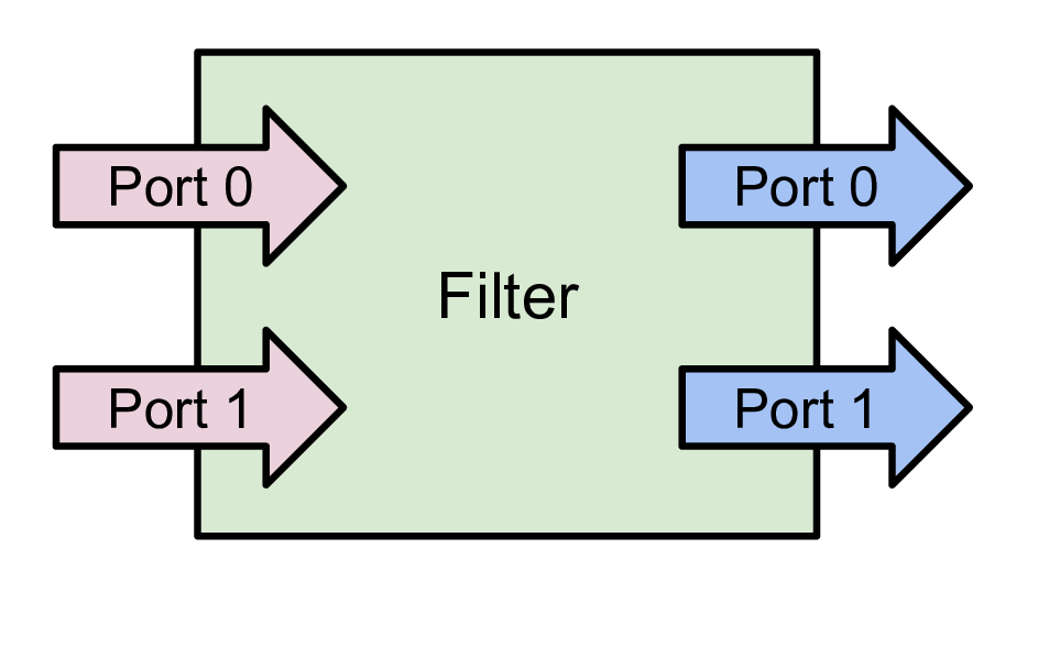
Fig. 5.1 A filter is a pipeline module with inputs and outputs.
Data enters a filter through the inputs. The filter transforms the data and
produces the resulting data on its outputs. A filter can have one or more input
and output ports. Each input port can optionally accept multiple input
connections.
An input port itself can optionally accept multiple input connections, e.g., the
AppendDatasets filter, which appends multiple datasets to create a single
dataset only has one input port (named Input ). However, that port can accept
multiple connections for each of the datasets to be appended . Filters define
whether a particular input port can accept one or many input connections.
Similar to readers, the properties on the filter allow you to control the
filtering algorithm. The properties available depend on the filter itself.
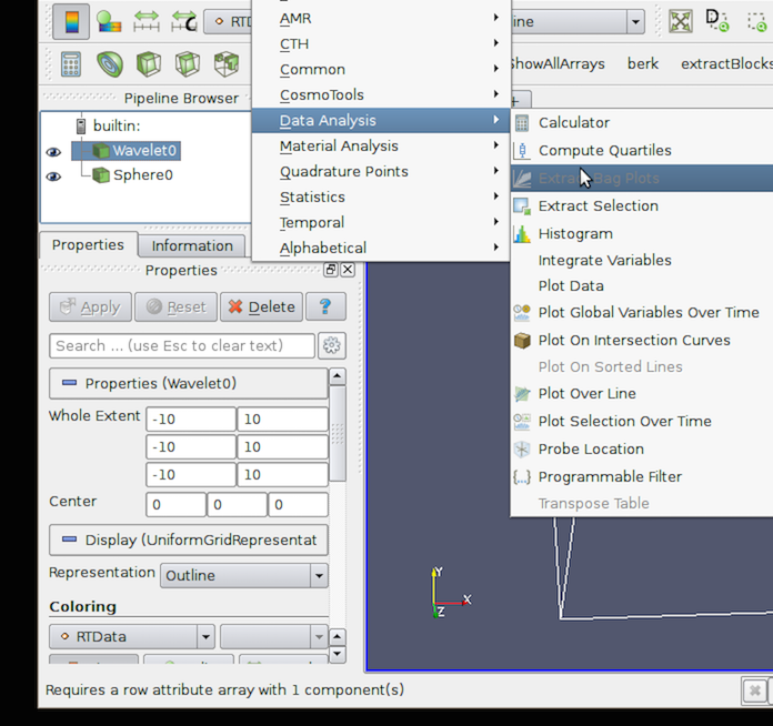
All available filters in paraview are listed under the Filters
menu. These are organized in various categories. To create a filter to transform
the data produced by a source or a reader, you select the source in the PipelineBrowser
to make it active, and then click on the corresponding menu item in the
Filters menu. If a menu item is disabled, it implies that the active source
does not produce data that can be transformed by this filter.
Did you know?
If a menu item in the Filters menu is disabled, it implies that the active
source(s) is not producing data of the expected type or the characteristics needed
by the filter. On Windows and Linux machines, if you hover over the disabled
menu item, the status bar will show the reason why the filter is not available.
When you create a filter, the active source is connected to the first input port
of the filter. Filters like AppendDatasets can take multiple input
connections on that input port. In such a case, to pass multiple pipeline
modules as connections on a single input port of a filter, select all the
relevant pipeline modules in the PipelineBrowser . You can select multiple
items by using the CTRL (or ⌘) and ⇧ key
modifiers. When multiple pipeline modules are selected, only the filters that
accept multiple connections on their input ports will be enabled in the
Filters menu.
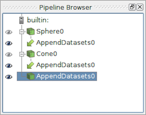
Fig. 5.2 The PipelineBrowser showing a pipeline with multiple input
connections. The AppendDatasets filter has two input connections on its
only input port, Sphere0 and Cone0 .
Most filters have just one input port. Hence, as soon as you click on the filter
name in the Filters menu, it will create a new filter instance and that
will show up in the PipelineBrowser . Certain filters, such as ResampleWithDataset , have multiple inputs that must be set up before the filter can be
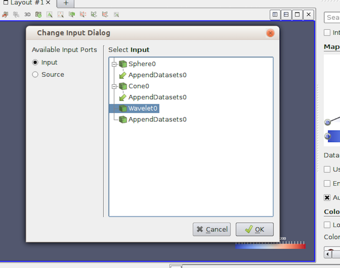
created. In such a case, when you click on the filter name, the ChangeInputDialog will pop up, as seen in Fig. 5.3.
This dialog allows you to select the pipeline modules to be
connected to each of the input ports. The active source(s) is connected by
default to the first input port. You are free to change those as well.
Fig. 5.3 The ChangeInputDialog is shown to allow you to pick inputs for
each of the input ports for a filter with multiple input ports. To use this
dialog, first select the InputPort you want to edit on the left side, and
select the pipeline module(s) that are to be connected to this input port.
Repeat the step for the other input port(s). If an input port can accept
multiple input connections, you can select multiple modules, just like in the
PipelineBrowser .
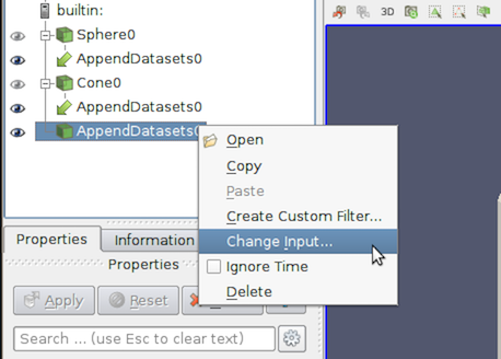
paraview allows you to change the inputs to a filter after the
filter has been created. To change inputs to a filter, right-click on the filter
in the PipelineBrowser to get the context menu, and then select ChangeInput... . This will pop up the same ChangeInputDialog as when creating a
filter with multiple input ports. You can use this dialog to set new inputs
for this filter.
Fig. 5.4 The context menu in the PipelineBrowser showing the option to
change inputs for a filter.
Did you know?
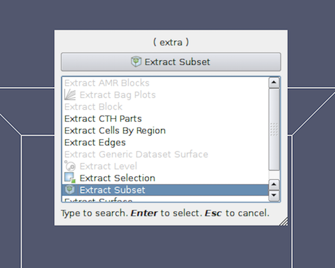
While the Filters menu is a handy way to create new filters, with the long list
of filters available in ParaView, manually finding a particular filter in this
menu can be very challenging. To make it easier, ParaView incorporates a quick
launch mechanism. When you want to create a new filter (or a source), simply type
CTRL + Space or Alt + Space. This will pop up
the quick-launch dialog. Now, start typing the name of the filter you want. As
you type, the dialog will update to show the filters and sources that match the
typed text. You can use the arrow keys to navigate and use the Enter key
to create the selected filter (or source). Press ⇧ while pressing Enter
to quickly apply the filter on creation, equivalent to creating the filter and then
clicking the Apply button. Note that filters may be disabled,
as was the case in the Filters menu but by default the selected item
will be the first enabled filter.
You can use Esc to clear the text you have typed so far. Hit the
Esc a second time, and the dialog will close without creating any new
filter.
Similar to paraview, the filter will use the active source(s) as
the input. Additionally, you can explicitly specify the input in the function
arguments.
To setup multiple input connections, you can specify the connections as follows:
>>> sphere=Sphere()>>> cone=Cone()# Simply pass the sources as a list to the constructor function.>>> appendDatasets=AppendDatasets(Input=[sphere,cone])>>> print(appendDatasets.Input)[<paraview.servermanager.Sphere object at 0x6d75f90>, <paraview.servermanager.Cone object at 0x6d75c50>]
Setting up connections to multiple input ports is similar to the multiple input
connections, except that you need to ensure that you name the input ports properly.
Changing inputs in Python is as simple as setting any other property on the
filter.
# For filter with single input connection>>>shrink.Input=cone# for filters with multiple input connects>>>appendDatasets.Input=[reader,cone]# to add a new input.>>>appendDatasets.Input.append(sphere)# to change multiple ports>>>resampleWithDataSet.Input=wavelet2>>>resampleWithDataSet.Source=cone
Filters provide properties that you can change to control the processing
algorithm employed by the filter. Changing and viewing properties on filters is
the same as with any other pipeline module, including readers and sources.
You can view and change these properties, when available, using the
Properties panel.
Section 1 covers how to effectively use the
Properties panel. Since this panel only shows the properties present on the
active source , you must ensure that the filter
you are interested in is active. To make the filter active, use the PipelineBrowser to click on the filter and select it.
With pvpython, the available properties are accessible as properties
on the filter object, and you can get or set their values by name (similar to
changing the input connections
(Section 5.3.3)).
# You can save the object reference when it's created.>>>shrink=Shrink()# Or you can get access to the active source.>>>Shrink()# <-- this will make the Shrink the active source.>>>shrink=GetActiveSource()# To figure out available properties, you can always use help.>>>help(shrink)HelponShrinkinmoduleparaview.servermanagerobject:classShrink(SourceProxy)|Shrink(**args)||TheShrinkfiltercausestheindividualcellsofadatasettobreakapartfromeachotherbymovingeachcell's points toward the centroid of the cell. (Thecentroidofacellistheaveragepositionofitspoints.)Thisfilteroperatesonanytypeofdatasetandproducesunstructuredgridoutput.||Methodresolutionorder:|Shrink|SourceProxy|Proxy|builtins.object||Methodsdefinedhere:||Initialize=aInitialize(self,connection=None,update=True)||----------------------------------------------------------------------|Datadescriptorsdefinedhere:||Input|ThispropertyspecifiestheinputtotheShrinkfilter.||ShrinkFactor|Thevalueofthispropertydetermineshowfarthepointswillmove.Avalueof0positionsthepointsatthecentroidofthecell;avalueof1leavesthemattheiroriginalpositions.....# To get the current value of a property:>>>sf=shrink.ShrinkFactor>>>printsf0.5# To set the value>>>shrink.ShrinkFactor=0.75
In the rest of this chapter, we will discuss some of the commonly used filters
in detail. They are grouped under categories based on the type of operation that they
perform.
These filters are used for extracting subsets from an input dataset. How this
subset is defined and how it is extracted depends on the type of the filter.
Clip is used to clip any dataset using either an implicit function (such as
a plane, sphere, or a box) or using values of a scalar data array in the input
dataset. A scalar array is a point or cell attribute array with a single
component. Clipping involves iterating over all cells in the input dataset and then
removing those cells that are considered outside of the space defined by
the implicit function or that have an attribute values less than the selected value.
For cells that straddle the clipping surface, these are clipped to pass
through the part of the cell that is truly inside the specified implicit
function (or greater than the scalar value).
This filter converts any dataset into an unstructured grid
(Section 3.1.7) or a multiblock of
unstructured grids (Section 3.1.10) in the case of composite
datasets.
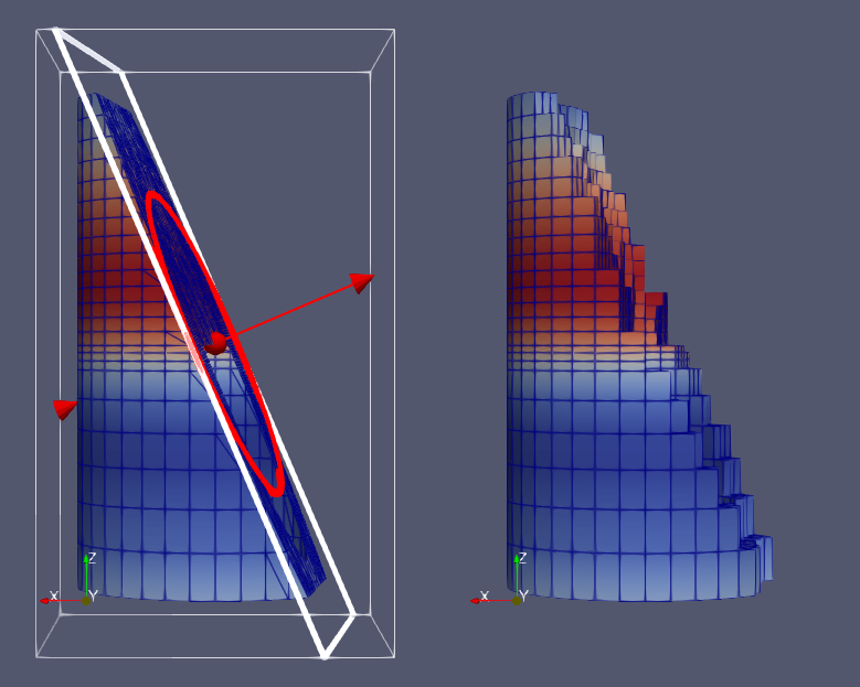
Fig. 5.5 Comparison between results produced by the Clip filter with
CrinkleClip unchecked (left) and checked (right) when clipping with an
implicit plane. The image on the left also shows the 3D widget used to
interactivly place the implicit plane for the clipping operation.
To create the Clip filter, access it through the Filters > Common or
the Filters > Alphabetical menus. This filter is also accessible from the
Common filters toolbar by clicking the button to create
this filter.
Fig. 5.6 The Common filters toolbar in paraview for quick
access to the commonly used filters.
On the Properties panel, you will see the available properties for this
filter. One of the first things that you should select is the ClipType .
ClipType is used to specify the type of implicit function to use for the
clipping operations. The available options include Plane , Box ,
Sphere , and Scalar . Selecting any one of these options will update
the panel to show properties that are used to define the implicit function, e.g.,
the Origin and the Normal for the Plane or the Center and
the Radius for the Sphere . If you select Scalar , the panel will let
you pick the data array and the value with which to clip. Remember, cells with the
data value greater than or equal to the selected value are considered in
and are passed through the filter.
Did you know?
When clipping with implicit functions, ParaView renders widgets in the active
view that you can use to interactively control the implicit function, called
3Dwidgets . As you interact with the 3D widget, the panel will update to
reflect the current values. The 3D widget is considered an aid and not as a part
of the actual visualization scene. Thus, if you change the active source and the
Properties panel navigates away from this filter, the 3D widget will
automatically be hidden.
The InsideOut option can be used to invert the behavior of this filter.
Basically, it flips the notion of what is considered inside and outside of the given
clipping space.
Check CrinkleClip if you don’t want this filter to truly clip cells on the
boundary, but want to preserve the input cell structure and to pass the entire cell on through the
boundary (Fig. 5.5).
This option is not available when clipping by Scalar .
This following script demonstrates various aspects of using the Clip filter
in pvpython.
# Create the Clip filter.>>>clip=Clip(Input=...)# Specify a 'ClipType' to use.>>>clip.ClipType='Plane'# You can also use the SetProperties API instead.>>>SetProperties(clip,ClipType='Plane')>>>print(clip.GetProperty('ClipType').GetAvailable())['Plane','Box','Sphere','Scalar']# To set the plane origin and normal>>>clip.ClipType.Origin=[0,0,0]>>>clip.ClipType.Normal=[1,0,0]# If you want to change to Sphere and set center and# radius, you can do the following.>>>clip.ClipType='Sphere'>>>clip.ClipType.Center=[0,0,0]>>>clip.ClipType.Radius=12# Using SetProperties API, the same looks like>>>SetProperties(clip,ClipType='Sphere')>>>SetProperties(clip.ClipType,Center=[0,0,0],Radius=12)# To set Crinkle clipping.>>>clip.Crinkleclip=1# For clipping with scalar, you pick the scalar array# and then the value as follows:>>>clip.ClipType='Scalar'>>>clip.Scalars=('POINTS','Temp')>>>clip.Value=100
# As always, to get the list of available properties on# the clip filter, use help()>>>help(clip)HelponClipinmoduleparaview.servermanagerobject:classClip(SourceProxy)|Clip(**args)||TheClipfiltercutsawayaportionoftheinputdatasetusinganimplicitfunction(animplicitdescription).Thisfilteroperatesonalltypesofdatasets,anditreturnsunstructuredgriddataonoutput.||Methodresolutionorder:|Clip|SourceProxy|Proxy|builtins.object||Methodsdefinedhere:||Initialize=aInitialize(self,connection=None,update=True)||----------------------------------------------------------------------|Datadescriptorsdefinedhere:||ClipType|Thispropertyspecifiestheparametersoftheclipfunction(animplicitdescription)usedtoclipthedataset.||Crinkleclip|Thisparametercontrolswhethertoextractentirecellsinthegivenregionorclipthosecellssoalloftheoutputwillstayonlyonthatsideofregion.||Exact|Ifthispropertyissetto1itwillcliptotheexactspecificationsforthe**Box**optiononly,otherwisetheclipwillonlyapproximatetheboxgeometry.Theexactclipisveryexpensiveasitrequiresgenerating6planeclips.Additionally,**Invert**mustbecheckedand**Crinkleclip**mustbeunchecked.||HyperTreeGridClipper|Thispropertyspecifiestheparametersoftheclipfunction(animplicitdescription)usedtoclipthehypertreegrid.||Input|ThispropertyspecifiesthedatasetonwhichtheClipfilterwilloperate.||Invert|Invertwhichpartofthegeometryisclipped....# To get help on a specific implicit function type, make it the active# ClipType and then use help()>>>clip.ClipType='Plane'>>>help(clip.ClipType)HelponPlaneinmoduleparaview.servermanagerobject:classPlane(Proxy)...
Common Errors
It is very easy to forget that clipping a structured dataset such as image
data can dramatically increase the memory requirements, since this filter will
convert the structured dataset into an unstructured grid due to the nature of
the clipping operation itself. For structured dataset, think about using
Slice or ExtractSubset filters instead, whenever appropriate. Those
are not entirely identical operations, but they are often sufficient.
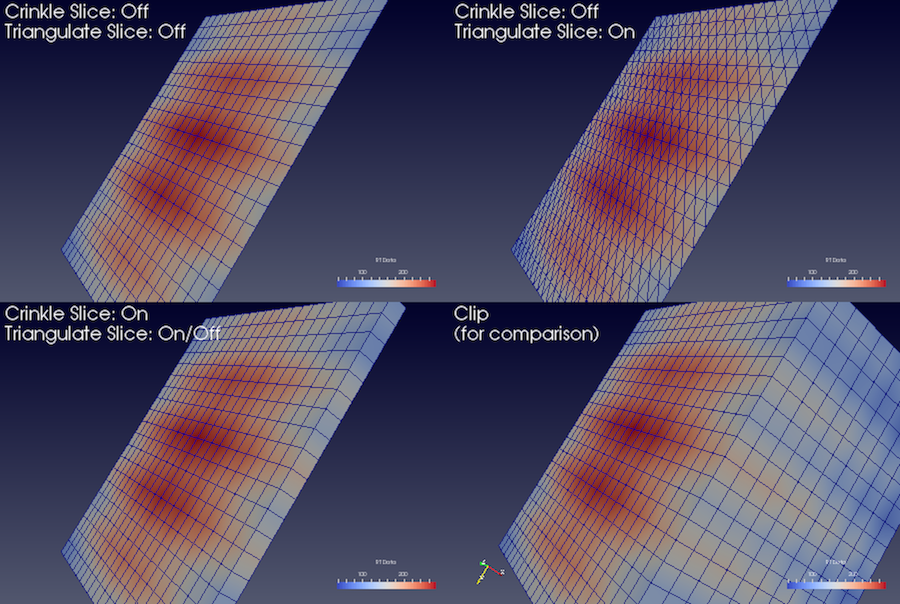
Fig. 5.7 Comparison between results produced by the Slice filter
when slicing image data with an implicit plane with different options.
The lower-left image shows the output produced by the Clip filter
when clipping with the same implicit function, for contrast.
The Slice filter slices through the input dataset with an implicit function
such as a plane, a sphere, or a box. Since this filter returns data elements along
the implicit function boundary, this is a dimensionality reducing filter (except
when crinkle slicing is enabled), i.e., if
the input dataset has 3D elements like tetrahedrons or hexahedrons, the output
will have 2D elements, line triangles, and quads, if any. While slicing through a
dataset with 2D elements, the result will be lines.
The properties available on this filter, as well as the way of setting this
filter up, is very similar to the Clip filter with a few notable
differences. What remains similar is the set up of the implicit function –
you have similar choices: Plane , Box , Sphere , and Cylinder , as well as the
option to toggle Crinkleslice (i.e., to avoid cutting through cells,
pass complete cells from the input dataset that intersects the implicit function).
What is different includes the lack of slicing by Scalar (for that, you
can use the Contour filter) and a new option, Triangulatetheslice .
Fig. 5.7
shows the difference in the generated meshes when various slice properties are
changed.
The Slice filter is more versatile than the Slice representation. First,
the Slice representation is available for image datasets only, whereas the
Slice filter can be used on any type of 3D dataset. Second, the representation
extracts a subset of the image consisting of a 2D slice oriented in the XY,
YZ, or XZ planes at the image voxel locations while the plane used by the filter
can be placed arbitrarily. Third, since the Slice representation always
shows a flat object and lighting may interfere with interpretation of data values
on the slice, lighting is not applied to the Slice representation. Lighting
is applied, however, to results from the Slice filter. Lastly, the Slice
representation may be faster than the filter to update and scrub through different
slices because it does not need to compute the intersection of a plane with cells
in the dataset.
In paraview, this filter can be created using the
button on the Common filters toolbar, besides the
Filters menu.
Fig. 5.8 The Properties panel for the ExtractSubset filter showing all
available properties (including the advanced properties).
For structured datasets such as
image datasets (Section 3.1.3), rectilinear grids
(Section 3.1.4), and
curvilinear grids (Section 3.1.5), ExtractSubset filter can be used to extract a region of interest or a subgrid. The
region to extract is specified using structured coordinates, i.e., the
\(i\), \(j\), \(k\) values. Whenever possible, this filter should be preferred over
Clip or Slice for structured datasets, since it preserves the input
data type. Besides extracting a subset, this filter can also be used to resample
the dataset to a coarser resolution by specifying the sample rate along each of
the structured dimensions.
This is one of the filters available on the Common filters toolbar
To specify the region of interest, use the VOI property. The values are
specified as min and max values for each of the structured dimensions (\(i\), \(j\),
\(k\),) in each row. SampleRateI , SampleRateJ ,
and SampleRateK specify the sub-sampling rate. Set it to a value greater than one to sub-sample.
IncludeBoundary is used to determine if the boundary slab should be
included in the extracted result, if the sub-sampling rate along that dimension
is greater than 1, and the boundary slab would otherwise have been skipped.
Fig. 5.9 Results from using the Threshold filter on the iron_protein.vtk dataset from ParaView’s testing data.
The Threshold filter extracts cells of the input dataset with scalar
values lying within the specified range, depending on the selected threshold method.
This filter operates on either point-centered or cell-centered data.
Any type of dataset can be used as input. The filter produces an unstructured grid output.
When thresholding with cell data, all cells that have scalars within the
specified range will be passed through the filter. When thresholding with point
data, cells with all points with scalar values within the range are passed
through if AllScalars is checked; otherwise, cells with any point
that passes the thresholding criteria are passed through.
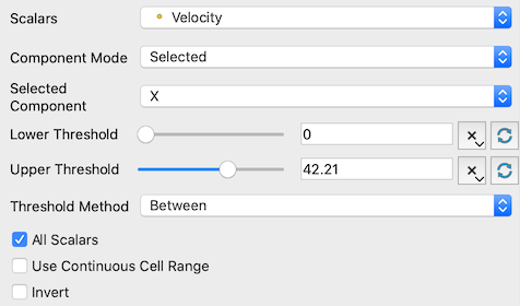
Fig. 5.10 The Properties panel for the Threshold filter.
This filter is represented as on the Common filters toolbar.
After selecting the Scalars with which to threshold from the combo-box, the
LowerThreshold and UpperThreshold values can be modified to specify the
range. If the range shown by the sliders is not sufficient, it is also possible
to manually type the values in the input boxes. The values are deliberately not
clamped to the current data range.
The threshold method can also be selected using the ThresholdMethod combo box:
Between: Extracts cells with scalar values between the LowerThreshold
and UpperThreshold.
BelowLowerThreshold: Extracts cells with scalar values smaller than the
LowerThreshold.
AboveUpperThreshold: Extracts cells with scalar values larger than the
UpperThreshold.
If the Scalars property is set to a vector array, the ComponentMode
property can be used to choose whether “All” components must pass the threshold test,
“Any” component needs to pass the threshold test, or if a “Selected” component
needs to pass the threshold test. If ComponentMode is “Selected”, the
SelectedComponent property designates which vector component needs to pass the
threshold test. Other components are not tested.
# Create the filter. If Input is not specified, the active source will be# used as the input.>>>threshold=Threshold(Input=...)# Here's how to select a scalar array.>>>threshold.Scalars=("POINTS","scalars")# The value is a tuple where the first value is the association: either "POINTS"# or "CELLS", and the second value is the name of the selected array.>>>print(threshold.Scalars)['POINTS','scalars']>>>print(threshold.Scalars.GetArrayName())'scalars'>>>print(threshold.Scalars.GetAssociation())'POINTS'# Different threshold methods are available and are set using one of the following:>>>threshold.ThresholdMethod="Between"# Uses both lower and upper values>>>threshold.ThresholdMethod="Below Lower Threshold"# Uses only lower value>>>threshold.ThresholdMethod="Above Upper Threshold"# Uses only upper value# The adequate threshold values are then specified as:>>>threshold.LowerThreshold=63.75>>>threshold.UpperThreshold=252.45
To determine the types of arrays available in the input dataset, and their
ranges, refer to the discussion on data information in
Section 3.3.
The IsoVolume filter is similar to Threshold in that you use this to
create an output dataset from an input where the cells that satisfy the
specified range are scalar values. In fact, the filter is identical to
Threshold when the cell data scalars are selected. For point data scalars,
however, this filter acts similar to the Clip filters when clipping with
scalars, in that cells are clipped along the iso-surface formed by the scalar range.
ExtractSelection is a general-purpose filter to extract selected elements
from a dataset. There are several ways of making selections in ParaView. Once
you have made the selection, this filter allows you to extract the selected
elements as a new dataset for further processing. We will cover this filter in
more detail when looking at selections in ParaView in
Section 6.6.
The Transform can be used to arbitrarily translate, rotate, and scale a
dataset. The transformation is applied by
scaling the dataset, rotating it, and then translating it
based on the values specified.
As this is a geometric manipulation filter, this filter does not affect
connectivity in the input dataset. While it tries to preserve the input dataset
type, whenever possible, there are cases when the transformed dataset can no
longer be represented in the same data type as the input. For example, with
image data (Section 3.1.3) and
rectilinear grids (Section 3.1.4) that are
transformed by rotation, the output dataset can be non-axis aligned and, hence,
cannot be represented as either data types. In such cases, the dataset is
converted to a structured, or curvilinear, grid
(Section 3.1.5). Since curvilinear grids are
not as compact as the other two, the need to store the results in a more general
data type implies a considerable increase in the memory footprint.
You can create a new Transform from the Filters > Alphabetical menu.
Once created, you can set the transform as the translation, rotation, and scale
to use utilizing the Properties panel. Similar to Clip , this filter also
supports using a 3D widget to interactively set the transformation.
Fig. 5.11 The Transform filter showing the 3D widget that can be used to interactively set the transform.
# To create the filter(if Input is not specified, the active source will be# used as the input).>>>transform=Transform(Input=...)# Set the transformation properties.>>>transform.Translate.Scale=[1,2,1]>>>transform.Transform.Translate=[100,0,0]>>>transform.Transform.Rotate=[0,0,0]
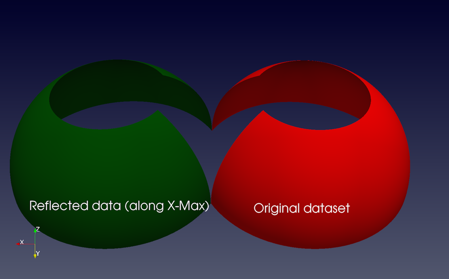
Fig. 5.12 The Reflect filter can be used to reflect a dataset along a specific axis plane.
Reflect can be used to reflect any dataset across an axis plane. You can
pick the axis plane to be one of the planes formed by the bounding box of the
dataset. For that, set Plane as XMin , XMax , YMin , YMax ,
ZMin , or ZMax . To reflect across an arbitrary axis plane,
select X , Y , or Z for the Plane property, and then set the
Center to the plane offset from the origin.
This filter reflects the input dataset and produces an unstructured grid
(Section 3.1.7). Thus, the same caveats for
Clip and Threshold filter apply here when dealing with structured
datasets.
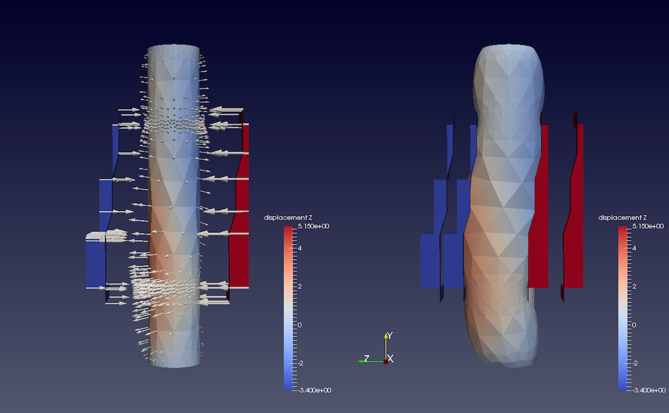
Fig. 5.13 The WarpByVector filter can be used to
displace points in original data shown on the left, using the
displacement vectors (indicated by arrow glyphs Section 5.8.1) to
produce the result shown on the right.
WarpByVector can be used to displace point coordinates in an input mesh
using vectors in the dataset itself. You select the vectors to use utilizing the
Vectors property on the Properties panel. ScaleFactor can be
used to scale the displacement applied.
WarpByScalar is similar to WarpByVector in the sense that it warps
the input mesh. However, it does so using a scalar array in the input dataset. The
direction of displacement can either be explicitly specified using the
Normal property, or you can check UseNormal to use normals at the
point locations.
Glyph is used to place markers or glyphs at point locations in the input
dataset. The glyphs can be oriented or scaled based on vector and
scalar attributes on those points.
To create this filter in paraview, you can use the Filters menu,
as well as the
button on the Common filters toolbar. You first select
the type of glyph using one of the options in GlyphType . The choices
include Arrow , Sphere , Cylinder , etc. Next, you select the point
arrays to use as the OrientationArray (selecting Noorientationarray
will result in the glyphs not being oriented). Similarly, you select a point array
to serve as the glyph ScaleArray (no scaling is performed if Noscalearray
is chosen).
If the ScaleArray is set to a vector array, the VectorScaleMode
property is available to select which properties of the vector should be used
to transform each glyph. If ScalebyMagnitude is chosen, then the glyph
at a point will be scaled by the magnitude of the vector at that point. If
ScalebyComponents is chosen, glyphs will be scaled separately in each
dimension by the vector component in that dimension.
Fig. 5.14 The Properties panel for the Glyph filter.
The ScaleFactor is used to apply a constant scaling to all the glyphs,
independent of the ScaleArray and VectorScaleMode properties.
Choosing a good scale factor depends on
several things including the bounds on the input dataset, the ScaleArray
and VectorScaleMode selected, and the range for the array selected as the
ScaleArray . You can use the button next to the ScaleFactor widget to have paraview
pick a usually reasonable scale factor value based on the current dataset and
scaling properties.
The Masking properties control which points from the input
dataset get glyphed. The GlyphMode controls how points are selected to be
glyphs (Fig. 5.15). The available options are as follows:
AllPoints : This selects all points in the input dataset for glyphing.
Use this mode with caution and only when the input dataset has relatively few
points. Since all points in the input dataset are glyphed, this can not only
cause visual clutter, but also clog up memory and take a long to time to
generate and render the glyphs.
EveryNthPoints : This elects every \(n^{th}\) point in the input dataset
for glyphing, where \(n\) can be specified using Stride . Setting
Stride to 1 will have the same effect as AllPoints .
UniformSpatialDistribution(BoundsBased) : This selects a random set of points. The
algorithm works by first computing up to MaximumNumberofSamplePoints
in the space defined by the bounding box of the input dataset. Then, points
in the input dataset that are close to the point in this set of sample points
are glyphed. The Seed is used to seed the random number generator used to
generate the sample points. This ensures that the random sample points are
reproducible and consistent.
UniformSpatialDistribution(SurfaceSampling) : Selects a random set of points
from the outer bounding surface of the input dataset. An inverse transform sampler
is used to find a 2D cell on the surface to sample and a point is uniformly sampled
from that cell.
UniformSpatialDistribution(VolumeSampling) : Similar to the surface sampling
mode described above, but the inverse transform sampler is used to find a 3D cell
from which a random point is uniformly sampled
Fig. 5.15 Comparison between various GlyphMode s when applied to the same
dataset generated by the Wavelet source.
Did you know?
The Glyph representation can be used for many of the same visualizations
where a Glyph filter might be used. It may offer faster rendering and consume
less memory than the Glyph filter with similar capabilities. In circumstances
where generating a 3D geometry is required, e.g., when exporting glyph geometry
to a file, the Glyph filter is required.
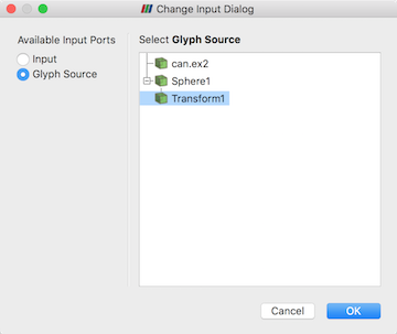
GlyphWithCustomSource is the same as Glyph , except that instead of a limited
set of GlyphType , you can select any data source producing a polygonal
dataset (Section 3.1.8) available in the PipelineBrowser . To use this filter, select the data source you wish to glyph in the
PipelineBrowser and attach this filter to it. You will be presented a dialog
where you can set the Input (which defaults to the source you selected) and
the GlyphSource .
Fig. 5.16 Setting the Input and GlyphSource in the GlyphWithCustomSource filter.
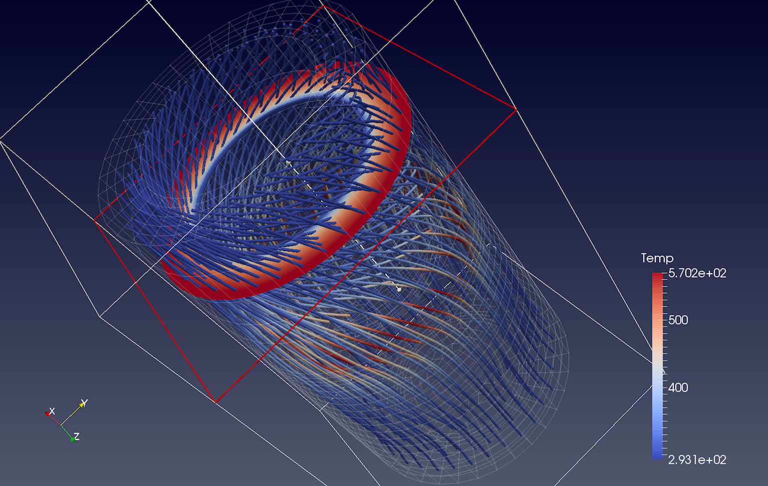
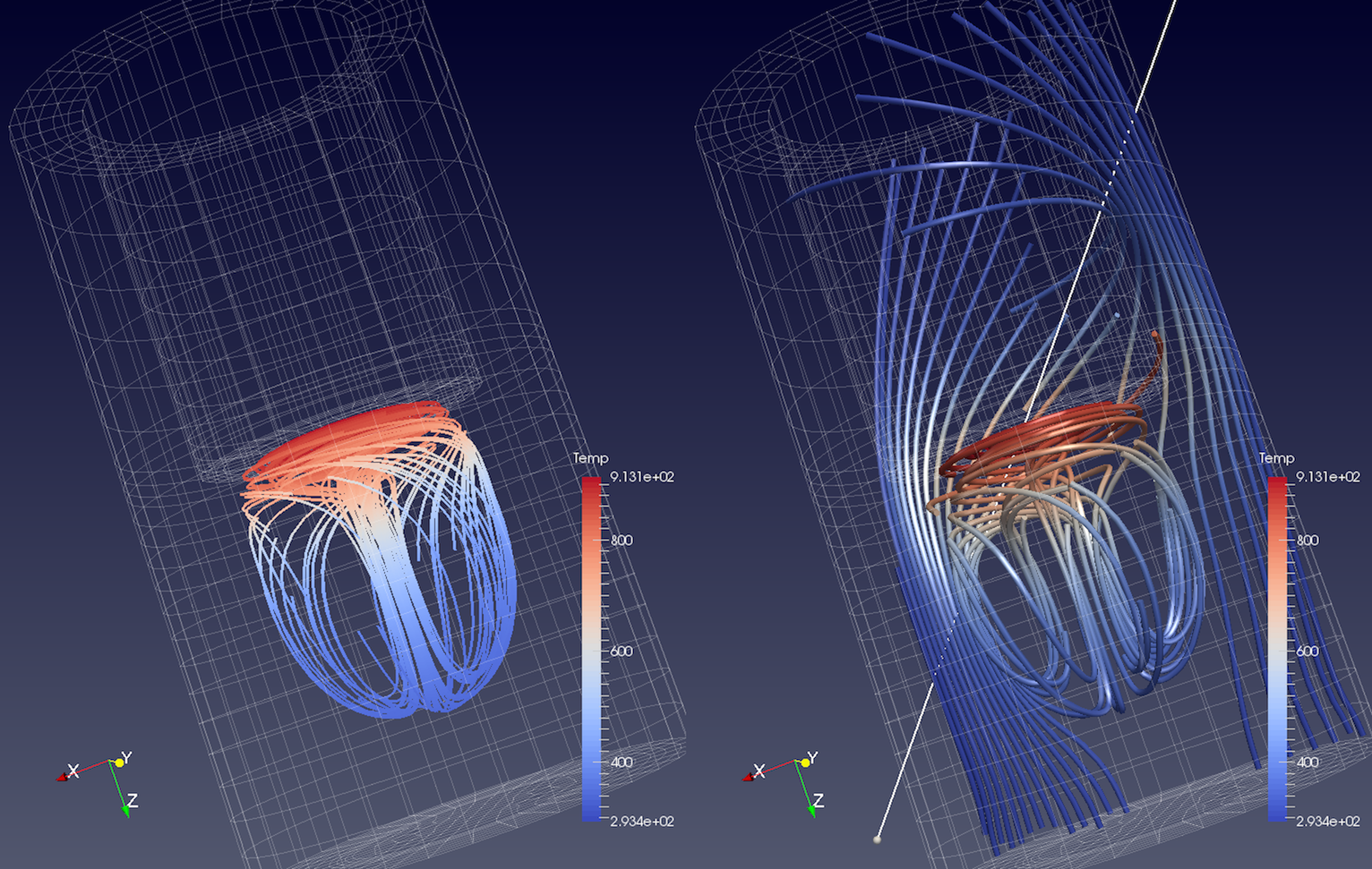
Fig. 5.17 Streamlines generated from the disk_out_ref.ex2 dataset
using the PointSource (left) and the HighResolutionLineSource
(right). On the left, we also added the Tube filter to the output of the
StreamTracer filter to generate 3D tubes rather than 1D polygonal lines,
which can be hard to visualize due to lack of shading.
The StreamTracer filter is used to generate streamlines for vector fields.
In visualization, streamlines refer to curves that are instanteneously
tangential to the the vector field in the dataset. They provide an indication of
the direction in which the particles in the dataset would travel at that instant
in time. The algorithm works by taking a set of points, known as seed
points, in the dataset and then integrating the streamlines starting at these seed
points.
In paraview, you can create this filter using the Filters
menu, as well as the button on the Common
filters toolbar. To use
this filter, you first select the attribute array to use as the Vectors for
generating the streamline. IntegrationParameters let you fine tune the
streamline integration by specifying the direction to integrate,
IntegrationDirection , as well as the type of integration algorithm to
use, IntegratorType . Advanced integration parameters are available in the
advanced view of the Properties panel that let you further tune the
integration, including specifying the step size and others. You use the
MaximumStreamlineLength to limit the maximum length for the streamline –
the longer the length, the longer the generated streamlines.
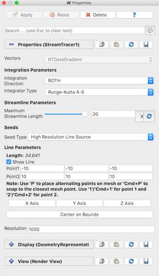
Fig. 5.18 The Properties panel showing the default properties for the
StreamTracer filter.
Seeds group lets you set how the seed points for generating the streamlines
are produced. You have two options: PointSource , which produces a point
clound around the user-specified Point based on the parameters specified,
and HighResolutionLineSource , which produces seed points along the user-specified
line. You can use the 3D widgets shown in the active RenderView
to interactively place the center for the point cloud or for defining the line.
Did you know?
The StreamTracer filter produces a polydata with 1D lines for each of the
generated streamlines. Since 1D lines cannot be shaded like surfaces in the
RenderView , you can get visualizations where it is hard to follow the
streamlines. To give the streamlines some 3D structure, you can apply the
Tube filter to the output of the streamlines. The properties on the
Tube filter let you control the thickness of the tubes. You can also vary
the thickness of the tubes based on data array, e.g., the magnitude of the
vector field at the sample points in the streamline!
A script using the StreamTracer filter in paraview typically
looks like this:
# find source>>>disk_out_refex2=FindSource('disk_out_ref.ex2')# create a new 'Stream Tracer'>>>streamTracer1=StreamTracer(Input=disk_out_refex2,SeedType='Point Source')>>>streamTracer1.Vectors=['POINTS','V']# init the 'Point Source' selected for 'SeedType'>>>streamTracer1.SeedType.Center=[0.0,0.0,0.07999992370605469]>>>streamTracer1.SeedType.Radius=2.015999984741211# show data in view>>>Show()# create a new 'Tube'>>>tube1=Tube(Input=streamTracer1)# Properties modified on tube1>>>tube1.Radius=0.1611409378051758# show the data from tubes in view>>>Show()
StreamTracer allows you to specify the seed points either as a point cloud
or as a line source. However, if you want to provide your own seed points from
another data producer, use the StreamTracerWithCustomSource . Similar to
GlyphWithCustomSource , this filter allows you to pick a second input
connection to use as the seed points.
Fig. 5.19 Streamlines generated from the disk_out_ref.ex2 dataset using the output of the Slice filter as the Source for seed points.
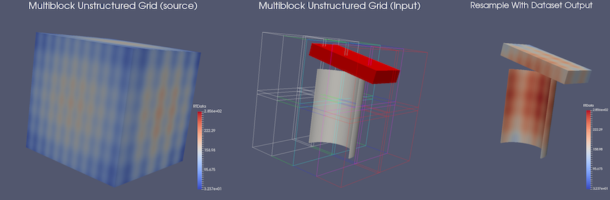
Fig. 5.20 An example of ResampleWithDataset . On the left is
a multiblock tetrahedra mesh ( Input ). The middle shows
a multiblock unstructured grid ( Source ). The outline of Input is
also shown in this view. The result of applying the filter is shown on
the right
ResampleWithDataset samples the point and cell attributes of one dataset
on to the points of another dataset. The two datasets are supplied to the
filter using its two input ports: Input , which is the dataset that
provides the attributes to resample, and Source , which is the dataset that
provides the points to sample at. This filter is available under the
Filters menu.
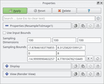
ResampleToImage is a specialization of ResampleWithDataset .
The filter takes one input and samples its point and cell attributes onto a
uniform grid of points. The bounds and extents of the uniform grid can be
specified using the properties panel. By default, the bounds are set to the
bounds of the input dataset. The output of the filter is an Image dataset.
Fig. 5.21 The Properties panel for ResampleToImage filter.
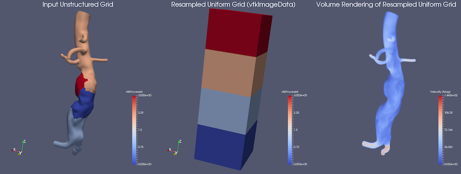
Fig. 5.22 An example of ResampleToImage . The left portion shows the input
(unstructured grid), and the middle displays the output image data.
On the right is a volume rendering of the resampled data.
Some operations can be performed more efficiently on uniform grid datasets.
Volume rendering is one such operation. The ResampletoImage filter can
be used to convert any dataset to Image data before performing such operations.
Probe samples the input dataset at a specific point location to obtain the
cell data attributes for the cell containing the point as well as the interpolated point
data attributes. You can either use the SpreadSheetView or the
Information panel to inspect the probed values. The probe location can be
specified using the interactive 3D widget shown in the active RenderView .
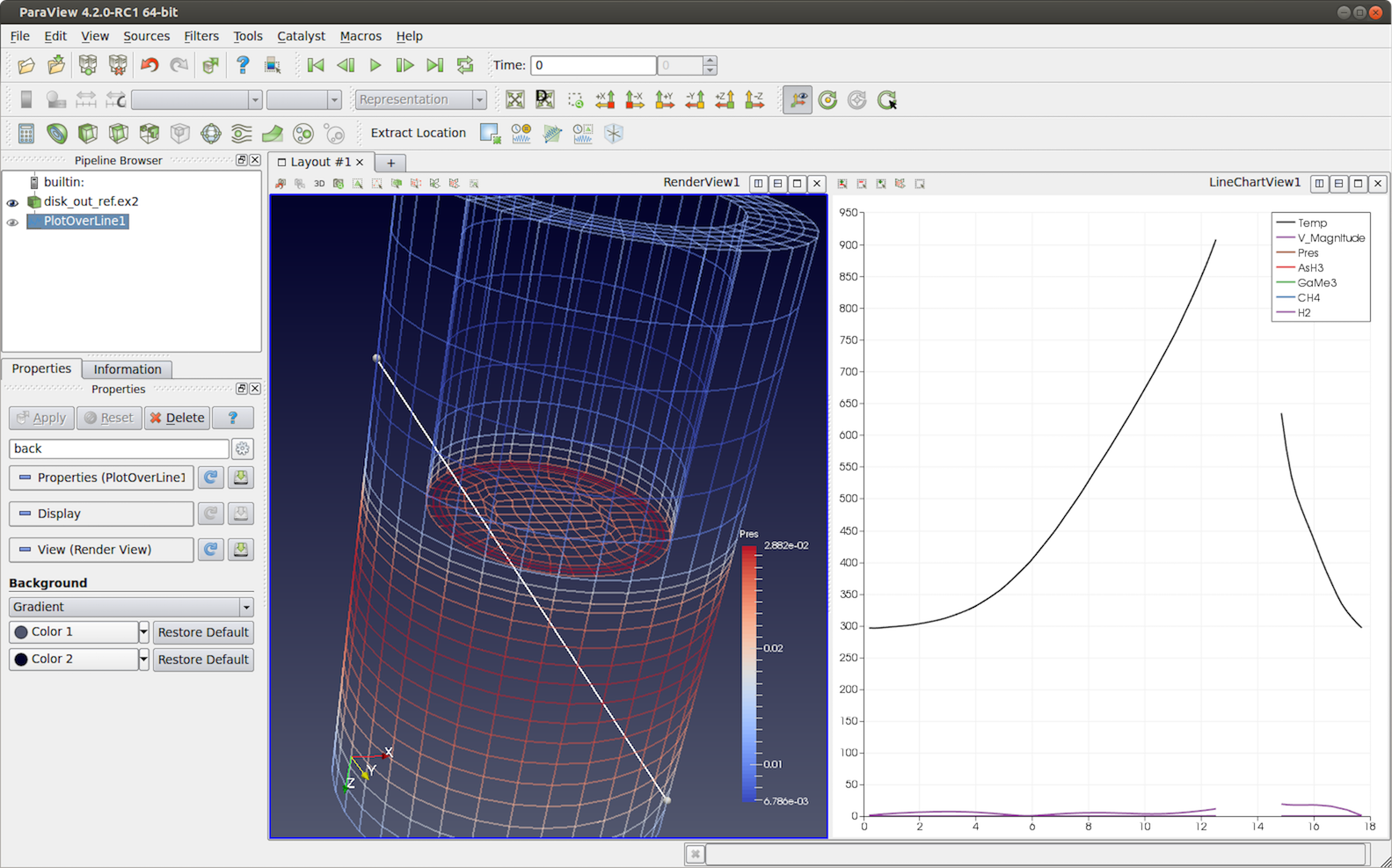
Fig. 5.23 The PlotOverLine filter applied to the disk_out_ref.ex2
dataset to plot values at sampled locations along the line. Gaps in the line correspond
to the locations in the input dataset where the line falls outside the dataset.
PlotOverLine will sample the input dataset along the specified line and
then plot the results in LineChartView . Internally, this filter uses the
same mechanism as the Probe filter, probing along the points in the
line to get the containing cell attributes and interpolated point attributes.
Using the Resolution property on the Properties panel, you can control
the number of sample points along the line.
The filters covered in this section are used to add new attribute arrays to the
dataset, which are typically used to add derived quantities to use in pipelines for
further processing.
The Calculator filter computes a new data array or new point coordinates as a
function of existing input arrays. If point-centered arrays are used
in the computation of a new data array, the resulting array will also be
point-centered. Similarly, computations using cell-centered arrays will produce
a new cell-centered array. If the function is computing point coordinates
(requested by checking the CoordinateResults property on the
Properties panel) , the
result of the function must be a three-component vector. The Calculator
interface operates similarly to a scientific calculator. In creating the
function to evaluate, the standard order of operations applies. Each of the
calculator functions is described below. Unless otherwise noted, enclose the
operand in parentheses using the ( and ) buttons.
Clear : Erase the current function.
/: Divide one scalar by another. The operands for this function are not required to be enclosed in parentheses.
*: Multiply two scalars, or multiply a vector by a scalar (scalar multiple). The operands for this function are not required to be enclosed in parentheses.
-: Negate a scalar or vector (unary minus), or subtract one scalar or vector from another. The operands for this function are not required to be enclosed in parentheses.
+: Add two scalars or two vectors. The operands for this function are not required to be enclosed in parentheses.
iHat , jHat , and kHat are vector constants representing unit vectors in the X, Y, and Z directions, respectively.
sin(x) : Compute the sine of a scalar.
cos(x) : Compute the cosine of a scalar.
tan(x) : Compute the tangent of a scalar.
abs(x) : Compute the absolute value of a scalar.
sqrt(x) : Compute the square root of a scalar.
asin(x) : Compute the arcsine of a scalar.
acos(x) : Compute the arccosine of a scalar.
atan(x) : Compute the arctangent of a scalar.
ceil(x) : Compute the ceiling of a scalar.
floor(x) : Compute the floor of a scalar.
sinh(x) : Compute the hyperbolic sine of a scalar.
cosh(x) : Compute the hyperbolic cosine of a scalar.
tanh(x) : Compute the hyperbolic tangent of a scalar.
x^y : Raise one scalar to the power of another scalar. The operands for this function are not required to be enclosed in parentheses.
exp(x) Raise \(e`\) to the power of a scalar.
dot(x,y) : Compute the dot product of two vectors x and y.
mag(x) : Compute the magnitude of a vector.
norm(x) : Normalize a vector. The operands are described below. The digits 0-9 and the decimal point are used to enter constant scalar values.
ln(x) : Compute the logarithm of a scalar to the base \(e\).
log10(x) : Compute the logarithm of a scalar to the base 10.
Additional operations are available in the Calculator filter that do not have buttons in the user interface, including:
avg(x,y,z,...) : Average of all the input arguments.
clamp(r0,x,r1) : Clamp x in range between r0 and r1.
cross(x,y) : Compute cross product of two vectors x and y.
equal(x,y) : Equality test between x and y using normalized epsilon.
erf(x) : Error function of x.
erfc(x) : Complimentary error function of x.
frac(x) : Fractional portion of x.
hypot(x,y) : Hypotenuse of x and y, equivalent of sqrt(x*x+y*y).
iclamp(r0,x,r1) : Inverse-clamp x outside of the range r0 and r1. If x is within the range it will snap to the closest bound.
inrange(r0,x,r1) : Returns true when x is within the range r0 and r1.
log1p(x) : Natural logarithm of 1 + x, where x is very small.
log2(x) : Base 2 logarithm of x.
logn(x,n) : Base N logarithm of x where n is a positive integer.
min(x,y) : Compute minimum of two scalars.
max(x,y) : Compute maximum of two scalars.
mul(z,y,z,...) : Multiply all the inputs together.
ncdf(x) : Normal cumulative distribution function.
not_equal(x,y) : Not-equal test between x and y using normalised epsilon.
pow(x,y) : x to the power of y.
root(x,n) : nth-root of x where n is a positive integer.
round(x) : Round x to the nearest integer
roundn(x,n) : Round x to n decimal places.
sgn(x) : Compute the sign of x: -1 where x < 0, +1 where x > 0, and 0 otherwise.
sum(x,y,z,...) : Sum of all the inputs.
trunc(x) : Integer portion of x.
acosh(x) : Inverse hyperbolic cosine of x expressed in radians.
asinh(x) : Inverse hyperbolic sine of x expressed in radians.
atan2(x,y) : Arc tangent of (x / y) expressed in radians.
atanh(x) : Inverse hyperbolic tangent of x expressed in radians.
cot(x) : Cotangent of x.
csc(x) : Cosecant of x.
sec(x) : Secant of x.
sinc(x) : Cardinal sine of x.
deg2rad(x) : Convert x from degrees to radians.
deg2grad(x) : Convert x from degrees to gradians.
rad2deg(x) : Convert x from radians to degrees.
grad2deg(x) : Convert x from gradians to degrees.
The following equalities and inequalities are available:
== or = : True only if x is strictly equal to y.
<> or != : True only if x does not equal y.
< : True only if x is less than y.
<= : True only if x is less than or equal to y.
> : True only if x is greater than y.
>= : True only if x is greater than or equal to y.
The following conditionals and boolean operators are available:
if(x,y,z) : If x evaluates to true, then y, otherwise z.
true : True state.
false : False state.
xandy : Logical and, true only if x and y are both true.
mand(x,y,z,...) : Multi-input logical and, true only if all arguments are true.
mor(x,y,z,...) : Multi-input logical or, true if any arguments are true.
xnandy : Logical nand, true only if either x or y is false.
xnory : Logical nor, true only if neither x or y is false.
notx : Logical not, evaluate to the opposite of the input boolean value.
xory : Logical or, true if either x or y is true.
xxory : Logical xor, true only if the logical state of x or y are different.
xxnory : True if and only if both logical inputs are the same.
The Scalars menu lists the names of the scalar arrays and the components of
the vector arrays of either the point-centered or
cell-centered data. The Vectors menu lists the names of the point-centered or
cell-centered vector arrays. The function will be computed for each point (or
cell) using the scalar or vector value of the array at that point (or cell). The
filter operates on any type of dataset, but the input dataset must have at
least one scalar or vector array. The arrays can be either point-centered or
cell-centered. The Calculator filter’s output is of the same dataset type as
the input.
Did you know?
It used to be a common use-case for the Calculator filter to convert three input
scalars into a vector array. For that, the Function would look something like:
\(scalar_x * iHat + scalar_y * jHat + scalar_z * kHat\).
Now, the Merge Vector Components filter provides a simpler way to do this
by simply selecting the three scalars to combine into a vector array.
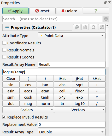
Fig. 5.24 The Properties panel for the Calculator filter showing the advanced properties.
The Properties panel provides access to several options for this filter.
Checking CoordinateResults , ResultNormals , or ResultTCoords
will set the computed array as the point coordinates, normals, or texture
coordinates, respectively. ResultArrayName is used to specify a name for
the computed array. The default is Result.
Sometimes, the expression can yield invalid values. To replace all invalid
values with a specific value, check the ReplaceInvalidResults checkbox and
then enter the value to use to replace invalid values using the
ReplacementValue . The output array data type is set with the ResultArrayType
property.
To ease the reuse of expressions, three helper buttons are also present to load an expression,
save the current one and inspect the list of already saved expressions from the ExpressionManager.
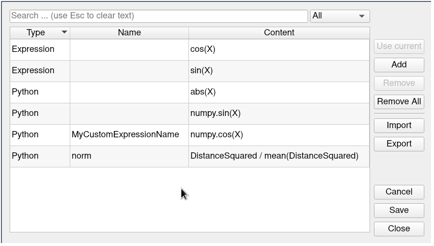
ParaView provides an ExpressionManager to ease the expression property configuration
by storing expressions, and giving quick access to them. Each expression can be named
and has an associated group so it is easy to filter Python expressions from others.
This feature comes in two parts:
From the PropertyPanel, the one-line property text entry is augmented with:
a drop down list to access existing expressions
a SaveCurrentExpression button
a shortcut to the ChooseExpression dialog
Fig. 5.25 Expression-related buttons in the Properties Panel.
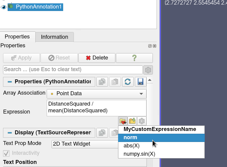
The ChooseExpression dialog, also accessible from the Tools > Manage Expressions menu item, is an editable and searchable list of the stored expressions. ParaView keeps track of them through the settings, but they can also be exported to a JSON file for backup and sharing.
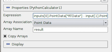
Fig. 5.27 The Properties Panel for PythonCalculator.
The PythonCalculator is similar to Calculator in that
it processes one or more input arrays based on an expression provided by the
user to produce a new output array. However, it uses Python (and
NumPy) to do the computation. Therefore, it provides more expressive
computational capabilities.
Specify whether to UseMultilineExpression, the Expression to use,
the ArrayAssociation to indicate the array association (PointData,
CellData, or FieldData), the name of output array (ArrayName),
a toggle that controls whether the input arrays are copied to the output
(CopyArray), and a ResultArrayType to specify the type of output
data array to store the calculated results in.
The PythonCalculator also integrated the ExpressionManager described in Section 5.9.2.
Start by creating a Sphere source and applying the PythonCalculator to it. As
the first expression, use the following and apply:
5
This should create an array name result in the output point data. Note
that this is an array that has a value of 5 for each point. When the expression
results in a single value, the calculator will automatically make a constant
array. Next, try the following:
Normals
Now, the result array should be the same as the input array Normals. As
described in detail later, various functions are available through the
calculator. For example, the following is a valid expression:
sin(Normals)+5
It is very important to note that the PythonCalculator has to produce one value
per point or cell depending on the Array Association parameter. Most of the
functions described here apply individually to all point or cell values and
produce an array the same dimensions as the input. However, some of them, such
as min() and max() , produce single values.
Common Errors
In the ProgrammableFilter , all the functions in
vtk.numpy_interface.algorithms are imported prior to executing the script.
As a result, some built-in functions, such as min and max , are
clobbered by that import. To use the built-in functions, import the import__builtin__
module and access those functions with, e.g.,
__builtin__.min and __builtin__.max
There are several ways of accessing input arrays within expressions. The
simplest way is to access it by name:
sin(Normals)+5
This is equivalent to:
sin(inputs[0].PointData['Normals'])+5
The example above requires some explanation. Here, inputs[0] refer to the
first input (dataset) to the filter. PythonCalculator can accept multiple
inputs. Each input can be accessed as inputs[0] , inputs[1] , … You
can access the point or cell data of an input using the .PointData or
.CellData qualifiers. You can then access individual arrays within the
point or cell data containers using the [] operator. Make sure to use
quotes or double-quotes around the array name. Arrays that have names with
certain characters (such as space, +, -, *, /) can only be accessed using this
method.
Certain functions apply directly on the input mesh. These filters expect an
input dataset as argument. For example,
area(inputs[0])
For data types that explicitly define the point coordinates, you can access the
coordinates array using the .Points qualifier. The following extracts the
first component of the coordinates array:
inputs[0].Points[:,0]
Note that for certain data types, mainly image data (uniform rectilinear grids)
and rectilinear grids, point coordinates are defined implicitly and cannot be
accessed as an array.
The PythonCalculator can be used to compare multiple datasets, as shown by
the following example.
Go to the Menu Bar, and select Edit > Reset Session to
clear the Pipeline.
Select Source > Mandelbrot, and then click
Apply, which will set up a default version of the Mandelbrot Set. The data for
this set are stored in a \(251 \times 251\) scalar array.
Select Source > Mandelbrot again, and then go to the Properties panel and
set the Maximum Number of Iterations to 50. Click Apply , which will set up
a different version of the Mandelbrot Set, represented by the same size array.
Hold the Shift key down and select both of the Mandelbrot entries in the
Pipeline Inspector, and then go to the Menu Bar, and select Filter >
Python Calculator. The two Mandelbrot entries will now be shown as linked, as
inputs, to the PythonCalculator .
In the Properties panel for the Python
Calculator filter, enter the following into the Expression box:
This expression specifies the difference between the second and the first
Mandelbrot arrays. The result is saved in a new array called results . The
prefixes in the names for the array variables, inputs[1] and
inputs[0] , refer to the first and second Mandelbrot entries, respectively,
in the Pipeline. PointData specifies that the inputs contain point values.
The quoted label 'Iterations' is the local name for these arrays. Click
Apply to initiate the calculation.
Click the Display tab in the PropertiesPanel for the PythonCalculator ,
and go to the first tab to the right of the Color by label. Select the
item results in that tab, which will cause the display window to the right to
show the results of the expression we entered in the PythonCalculator . The
scalar values representing the difference between the two Mandelbrot arrays are
represented by colors that are set by the current color map (click the Edit
button to open a detailed editor for the current color map).
There are a few things to note:
PythonCalculator will always copy the mesh from the first input to its output.
All operations are applied point-by-point. In most cases, this requires
that the input meshes (topology and geometry) are the same. At the least, it
requires that the inputs have the same number of points and cells.
In parallel execution mode, the inputs have to be distributed exactly the
same way across processes.
The PythonCalculator supports all of the basic arithmetic operations using the
\(+\), \(-\), \(*\) and \(/\) operators. These are always applied element-by-element to
point and cell data including scalars, vectors, and tensors. These operations
also work with single values. For example, the following adds 5 to all
components of all Normals.
Normals+5
The following adds 1 to the first component, 2 to the second component, and 3 to
the third component:
Normals+[1,2,3]
This is specially useful when mixing functions that return single values. For
example, the following normalizes the Normals array:
A common use case in a calculator is to work on one component of an array. This
can be accomplished with the following:
Normals[:,0]
The expression above extracts the first component of the Normals vector. Here,
: is a placeholder for “all elements”. One element can be extracted by replacing
: with an index. For example, the following creates a constant array from the
first component of the normal of the first point:
Normals[0,0]
Alternatively, the following assigns the normal of the first point to all points:
Normals[0,:]
It is also possible to create a vector array from two or three scalar arrays using the make_vector() function:
make_vector(velocity_x,velocity_y,velocity_z)
For temporal datasets, you also have access to the dataset timestep index or time value
in the expression as t_index or time_index , and t_value or time_value
respectively. When dealing with multiple inputs, you can specify the same variable names scoped on the
appropriate input e.g. inputs[0].t_index .
The locations of points are available in the Points variable for datasets that define explicit points positions.
In some datasets, field data is used to store global data values not associated with cells or points.
To use field data in a PythonCalculator expression, access it with the FieldData dictionary
available in the input as in the following example:
Under the cover, the PythonCalculator uses NumPy. All arrays in the
expression are compatible with NumPy arrays and can be used where NumPy arrays
can be used. For more information on what you can do with these arrays, consult
with the NumPy references [NumPydevelopers].
The following is a list of functions available in the PythonCalculator .
Note that this is a partial list, since most of the NumPy and SciPy functions
can be used in the PythonCalculator . Many of these functions can take
single values or arrays as argument.
abs(x) : Returns the absolute value(s) of \(x\).
add(x,y) : Returns the sum of two values. \(x\) and \(y\) can be single values or arrays. This is the same as \(x+y\).
area(dataset) : Returns the surface area of each cell in a mesh.
aspect(dataset) : Returns the aspect ratio of each cell in a mesh.
aspect_gamma(dataset) : Returns the aspect ratio gamma of each cell in a mesh.
condition(dataset) : Returns the condition number of each cell in a mesh.
cross(x,y) : Returns the cross product for two 3D vectors from two arrays of 3D vectors.
curl(array) : Returns the curl of an array of 3D vectors.
divergence(array) : Returns the divergence of an array of 3D vectors.
divide(x,y) : Element-by-element division. \(x\) and \(y\) can be single
values or arrays. This is the same as math:frac{x}{y}.
det(array) : Returns the determinant of an array of 2D square matrices.
determinant(array) : Returns the determinant of an array of 2D square matrices.
diagonal(dataset) : Returns the diagonal length of each cell in a dataset.
dot(a1,a2) : Returns the dot product of two scalars/vectors of two array of scalars/vectors.
eigenvalue(array) : Returns the eigenvalue of an array of 2D square matrices.
eigenvector(array) : Returns the eigenvector of an array of 2D square matrices.
exp(x) : Returns \(e^x\).
gradient(array) : Returns the gradient of an array of
scalars or vectors.
inv(array) : Returns the inverse an array of 2D square matrices.
inverse(array) : Returns the inverse of an array of 2D square matrices.
jacobian(dataset) : Returns the jacobian of an array of 2D square matrices.
laplacian(array) : Returns the jacobian of an array of scalars.
ln(array) : Returns the natural logarithm of an array of scalars/vectors/tensors.
log(array) : Returns the natural logarithm of an array of scalars/vectors/tensors.
log10(array) : Returns the base 10 logarithm of an array of scalars/vectors/tensors.
make_point_mask_from_NaNs(dataset,array) : This function will create a ghost array corresponding to an input with NaN values. For each NaN value, the output array will have a corresponding value of vtk.vtkDataSetAttributes.HIDDENPOINT . These values are also combined with any ghost values that the dataset may have.
make_cell_mask_from_NaNs(dataset,array) : This function will create a ghost array corresponding to an input with NaN values. For each NaN value, the output array will have a corresponding value of vtk.vtkDataSetAttributes.HIDDENCELL . These values are also combined with any ghost values that the dataset may have.
max(array) : Returns the maximum value of the array as a single value. In parallel, compute the max accross processes.
max_angle(dataset) : Returns the maximum angle of each cell in a dataset.
mag(a) : Returns the magnitude of an array of scalars/vectors.
mean(array) : Returns the mean value of an array of scalars/vectors/tensors. In parallel, compute the mean accross processes.
min(array) : Returns the minimum value of the array as a single value. In parallel, compute the min accorss processes.
min_angle(dataset) : Returns the minimum angle of each cell in a dataset.
mod(x,y) : Same as remainder \((x, y)\).
multiply(x,y) : Returns the product of \(x\) and \(y\). \(x\) and \(y\) can be
single values or arrays. Note that this is an element-by-element operation when
\(x\) and \(y\) are both arrays. This is the same as \(x \times y\).
negative(x) : Same as \(-x\).
norm(a) : Returns the normalized values of an array of scalars/vectors.
power(x,a) : Exponentiation of \(x\) with \(a\). Here, both \(x\) and \(a\) can
either be a single value or an array. If \(x\) and \(y\) are both arrays, a one-by-one
mapping is used between two arrays.
reciprocal(x) : Returns \(\frac{1}{x}\).
remainder(x,y) : Returns \(x - y \times floor(\frac{x}{y})\). \(x\) and \(y\) can be single values or arrays.
rint(x) : Rounds \(x\) to the nearest integer(s).
shear(dataset) : Returns the shear of each cell in a dataset.
skew(dataset) : Returns the skew of each cell in a dataset.
square(x) : Returns \(x*x\).
sqrt(x) : Returns \(\sqrt[2]{x}\).
strain(array) : Returns the strain of an array of 3D vectors.
subtract(x,y) : Returns the difference between two values. \(x\) and
y can be single values or arrays. This is the same as \(x - y\).
surface_normal(dataset) : Returns the surface normal of each cell in a dataset.
trace(array) : Returns the trace of an array of 2D square matrices.
volume(dataset) : Returns the volume normal of each cell in a dataset.
vorticity(array) : Returns the vorticity/curl of an array of 3D vectors.
vertex_normal(dataset) : Returns the vertex normal of each point in a dataset.
The Gradient filter computes the gradient of a cell or point data array for
any type of dataset.
For unstructured grids, the gradient for cell data corresponds to the cell derivatives.
For point data, the gradient at a given point is computed as the average of the
derivatives of the cells to which the point belongs.
For structured grids, the gradient is computed using central differencing, except
on the boundary of the dataset where forward and backward differencing is used for
the boundary elements.
This filter can optionally compute the divergence, vorticity (also known as the
curl), and Q-criterion. A 3-component array is required in order to compute these
quantities. By default, only the gradient computation is enabled.
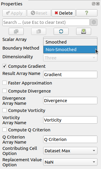
In the case of a uniform rectilinear grid (see Section 3.1.3),
a specific implementation which efficiently computes the gradient of point data arrays
is also available. This implementation extends the use of central differencing
on the boundary elements after duplication of the boundary values. To activate
this option, set the BoundaryMethod property to Smoothed, as shown in
Fig. 5.28.
Fig. 5.28 The Properties Panel for the Gradient filter applied to a uniform
structured grid.
The MeshQuality filter creates a new cell array containing a geometric
measure of each cell’s fitness. Different quality measures can be chosen for
different cell shapes.
TriangleQuality indicates which quality measure will be used to evaluate
triangle quality. The RadiusRatio is the size of a circle circumscribed by a
triangle’s three vertices divided by the size of a circle tangent to a triangle’s three
edges. The EdgeRatio is the ratio of the longest edge length to the shortest
edge length.
QuadQuality indicates which quality measure will be used to evaluate
quad cells.
TetQuality indicates which quality measure will be used to evaluate
tetrahedral quality. The RadiusRatio is the size of a sphere circumscribed by a
tetrahedron’s four vertices divided by the size of a circle tangent to a
tetrahedron’s four faces. The EdgeRatio is the ratio of the longest edge length to
the shortest edge length. The CollapseRatio is the minimum ratio of height of a
vertex above the triangle opposite it, divided by the longest edge of the
opposing triangle across all vertex/triangle pairs.
HexQualityMeasure indicates which quality measure will be used to evaluate
quality of hexahedral cells.
This includes the ProgrammableFilter and ProgrammableSource . For
these filters/sources, you can add Python code to do the data generation or
processing. We’ll cover writing Python code for these in
Section 5.
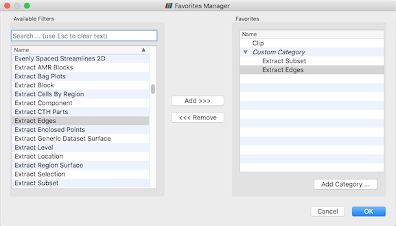
If you use some filters more than others, you can organize them in the Filters > Favorites menu.
This can be done from the context menu in the pipeline or through the Filters > Manage Favorites
menu as shown in Fig. 5.29. In this dialog you can create categories and
subcategories. It supports drag’n’drop operation to sort and move filters and categories.
Moreover, Favorites are highlighted in the other filter submenus on supported platforms.
Favorites are saved in user settings so they can be used in other subsequent ParaView sessions.
Fig. 5.29 The Favorites Manager dialog. Left: the list of available filters. Right: the favorites, organized into categories.
The pipeline model that ParaView presents is very convenient for exploratory
visualization. The loose coupling between components provides a very flexible
framework for building unique visualizations, and the pipeline structure allows
you to tweak parameters quickly and easily.
The downside of this coupling is that it can have a larger memory footprint.
Each stage of this pipeline maintains its own copy of the data. Whenever
possible, ParaView performs shallow copies of the data so that different stages
of the pipeline point to the same block of data in memory. However, any filter
that creates new data or changes the values or topology of the data must
allocate new memory for the result. If ParaView is filtering a very large mesh,
inappropriate use of filters can quickly deplete all available memory.
Therefore, when visualizing large datasets, it is important to understand the
memory requirements of filters.
Please keep in mind that the following advice is intended only for when dealing
with very large amounts of data and the remaining available memory is low. When
you are not in danger of running out of memory, the following advice is not
relevant.
When dealing with structured data, it is absolutely important to know what
filters will change the data to unstructured. Unstructured data has a much
higher memory footprint, per cell, than structured data because the topology
must be explicitly written out. There are many filters in ParaView that will
change the topology in some way, and these filters will write out the data as an
unstructured grid, because that is the only dataset that will handle any type of
topology that is generated. The following list of filters will write out a new
unstructured topology in its output that is roughly equivalent to the input.
These filters should never be used with structured data and should be used with
caution on unstructured data.
Append Datasets
Extract Edges
Subdivide
Append Geometry
Linear Extrusion
Tessellate
Clean
Loop Subdivision
Tetrahedralize
Clean to Grid
Reflect
Triangle Strips
Connectivity
Rotational Extrusion
Triangulate
D3
Shrink
Delaunay 2D/3D
Smooth
Technically, the Ribbon and Tube filters should fall into this list.
However, as they only work on 1D cells in poly data, the input data is usually
small and of little concern.
This similar set of filters also outputs unstructured grids, but also tends to
reduce some of this data. Be aware though that this data reduction is often
smaller than the overhead of converting to unstructured data. Also note that the
reduction is often not well balanced. It is possible (often likely) that a
single process may not lose any cells. Thus, these filters should be used with
caution on unstructured data and extreme caution on structured data.
Clip
Extract Selection
Decimate
Quadric Clustering
Extract Cells by Region
Threshold
Similar to the items in the preceding list, ExtractSubset performs data
reduction on a structured dataset, but also outputs a structured dataset. So the
warning about creating new data still applies, but you do not have to worry
about converting to an unstructured grid.
This next set of filters also outputs unstructured data, but it also performs a
reduction on the dimension of the data (for example 3D to 2D), which results in
a much smaller output. Thus, these filters are usually safe to use with
unstructured data and require only mild caution with structured data.
Cell Centers
Mask Points
Contour
Outline Curvilinear DataSet
Extract CTH Parts
Slice
Extract Surface
Stream Tracer
Feature Edges
The filters below do not change the connectivity of the data at all. Instead,
they only add field arrays to the data. All the existing data is shallow copied.
These filters are usually safe to use on all data.
Block Ids
Point Data to Cell Data
Calculator
Process Ids
Cell Data to Point Data
Random Vectors
Curvature
Resample with Dataset
Elevation
Surface Flow
Surface Normals
Surface Vectors
Gradient
Texture Map to…
Level Scalars
Transform
Median
Warp By Scalar
Mesh Quality
Warp By Vector
This final set of filters either add no data to the output (all data of
consequence is shallow copied) or the data they add is generally independent of
the size of the input. These are almost always safe to add under any
circumstances (although they may take a lot of time).
Annotate Time
Outline Corners
Append Attributes
Plot Global Variables Over Time
Extract Block
Plot Over Line
Glyph
Plot Selection Over Time
Group Datasets
Probe Location
Histogram
Temporal Shift Scale
Integrate Variables
Temporal Snap-to-Time-Steps
Normal Glyphs
Temporal Statistics
Outline
There are a few special case filters that do not fit well into any of the
previous classes. Some of the filters, currently TemporalInterpolator and
ParticleTracer , perform calculations based on how data changes over time.
Thus, these filters may need to load data for two or more instances of time,
which can double or more the amount of data needed in memory. The TemporalCache filter will also hold data for multiple instances of time. Keep in mind
that some of the temporal filters such as the Temporal Statistics and the
filters that plot over time may need to iteratively load all data from disk.
Thus, it may take an impractically long amount of time even if does not require
any extra memory.
The ProgrammableFilter is also a special case that is impossible to
classify. Since this filter does whatever it is programmed to do, it can fall
into any one of these categories.
When dealing with large data, it is best to cull out data whenever possible and
do so as early as possible. Most large data starts as 3D geometry and the
desired geometry is often a surface. As surfaces usually have a much smaller
memory footprint than the volumes that they are derived from, it is best to
convert to a surface early on. Once you do that, you can apply other filters in
relative safety.
A very common visualization operation is to extract isosurfaces from a volume
using the Contour filter. The Contour filter usually outputs geometry much
smaller than its input. Thus, the Contour filter should be applied early if
it is to be used at all. Be careful when setting up the parameters to the
Contour filter because it still is possible for it to generate a lot of
data which can happen if you specify many isosurface values. High frequencies
such as noise around an isosurface value can also cause a large, irregular
surface to form.
Another way to peer inside of a volume is to perform a Slice on it. The
Slice filter will intersect a volume with a plane and allow you to see the
data in the volume where the plane intersects. If you know the relative location
of an interesting feature in your large dataset, slicing is a good way to view
it.
If you have little a priori knowledge of your data and would like to
explore the data without the long memory and processing time for the full
dataset, you can use the ExtractSubset filter to subsample the data. The
subsampled data can be dramatically smaller than the original data and should
still be well load balanced. Of course, be aware that you may miss small
features if the subsampling steps over them and that once you find a feature you
should go back and visualize it with the full dataset.
There are also several features that can pull out a subset of a volume:
Clip , Threshold , ExtractSelection , and ExtractSubset can
all extract cells based on some criterion. Be aware, however, that the extracted
cells are almost never well balanced; expect some processes to have no cells
removed. All of these filters, with the exception of ExtractSubset , will
convert structured data types to unstructured grids. Therefore, they should not
be used unless the extracted cells are of at least an order of magnitude less
than the source data.
When possible, replace the use of a filter that extracts 3D data with one that
will extract 2D surfaces. For example, if you are interested in a plane through
the data, use the Slice filter rather than the Clip filter. If you are
interested in knowing the location of a region of cells containing a particular
range of values, consider using the Contour filter to generate surfaces at
the ends of the range rather than extract all of the cells with the
Threshold filter. Be aware that substituting filters can have an effect on
downstream filters. For example, running the Histogram filter after
Threshold will have an entirely different effect than running it after the
roughly equivalent Contour filter.
 button to create
this filter.
button to create
this filter.
 button on the
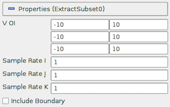
 To specify the region of interest, use the
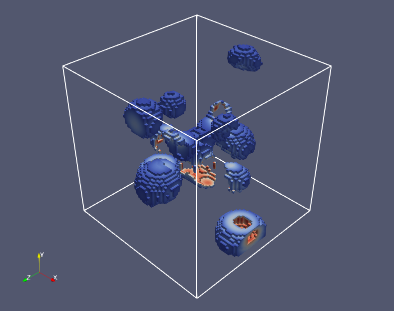
 on the
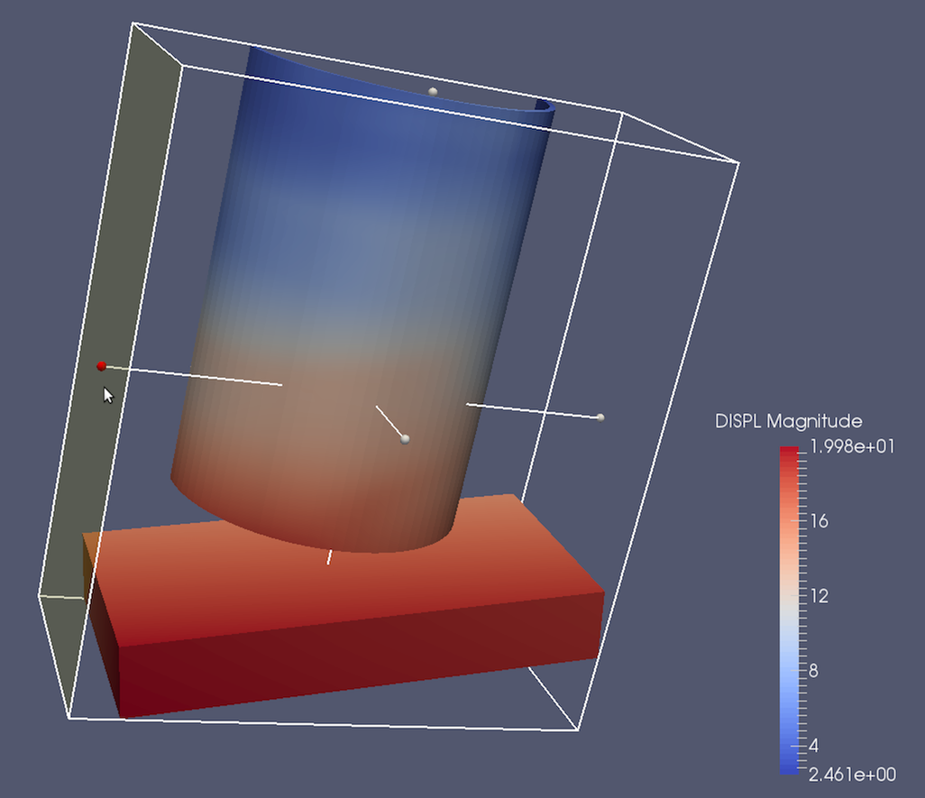
 button on the
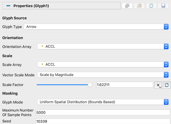
 button next to the
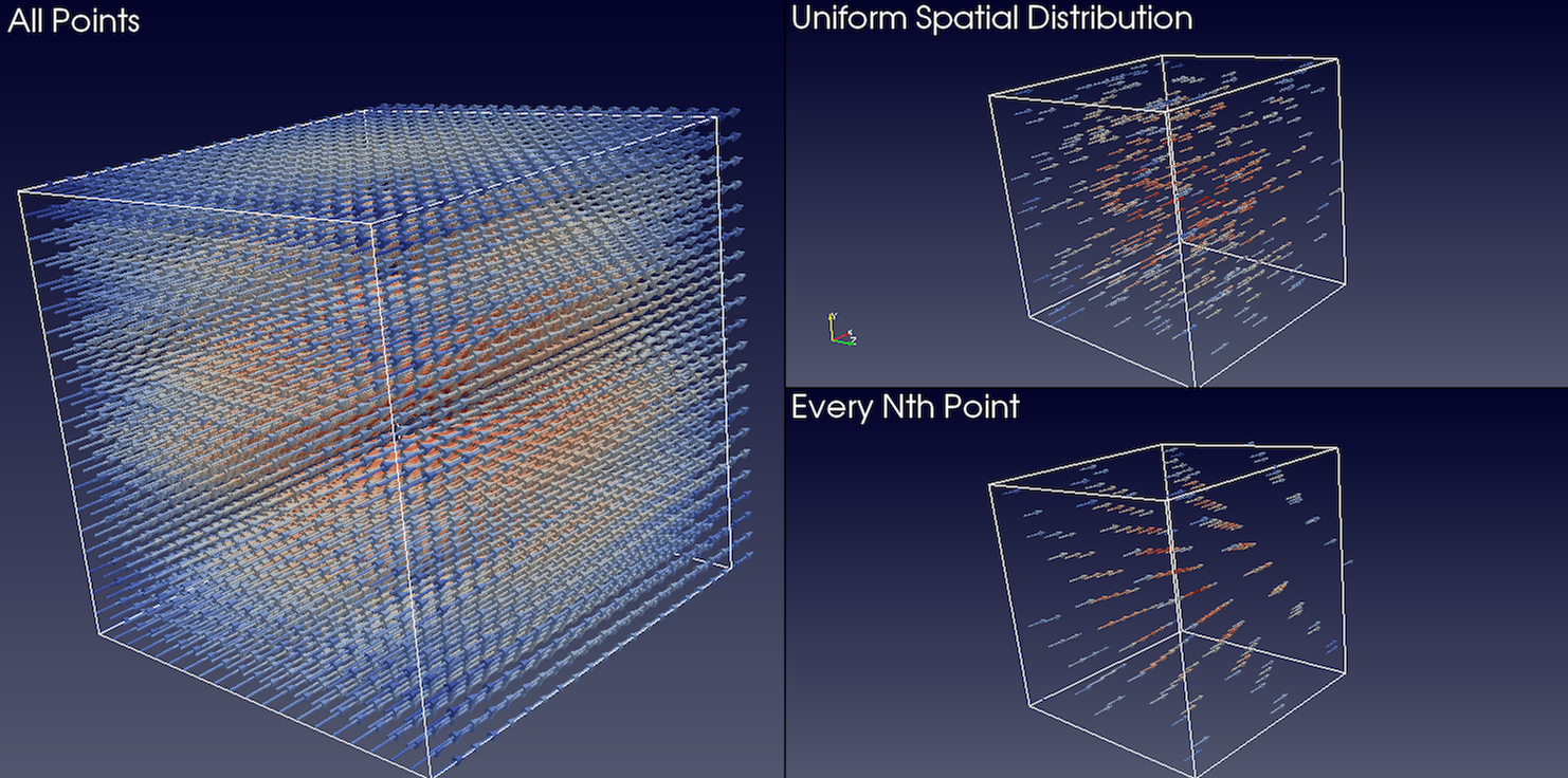
 button on the